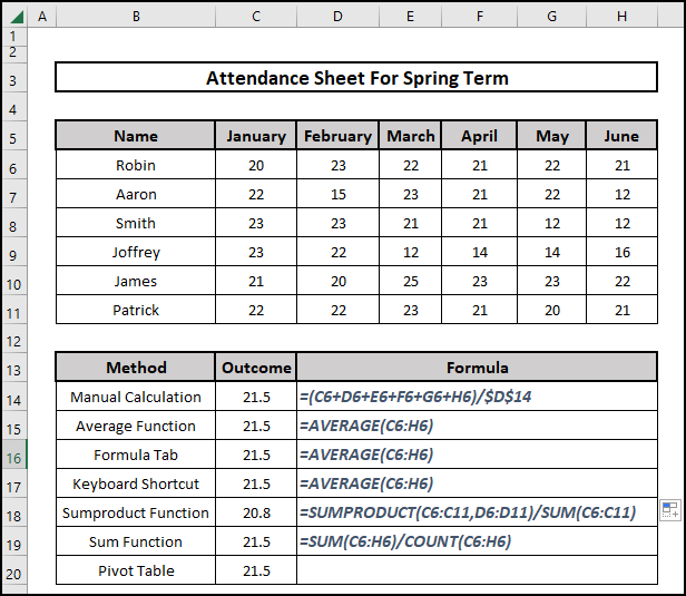
Almost every educational institution or Office needs to keep a record of the attendance of their students or employees. In school, it is necessary for preparing the final result of a student. In the office, this record helps us to prepare the salary sheet. So making an attendance formula is very common. We can easily do this task in Excel. In this article, we are going to learn 7 simple ways to prepare the average attendance formula in Excel. In some methods, we will use features like Formula Tab, Pivot Table, Keyboard shortcuts, etc. We will also imply different Excel functions such as AVERAGE, SUM & COUNT, SUMPRODUCT, etc. We can quickly take a glance at the methods and outcome of this article from the snapshot given below.
📁 Download Excel File
Download the practice file from here.
Learn to Calculate Average Attendance with Formula in Excel with These 5 Methods
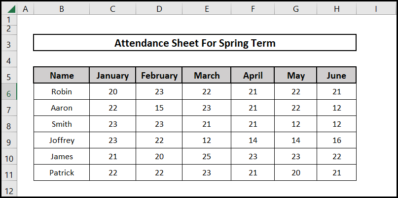
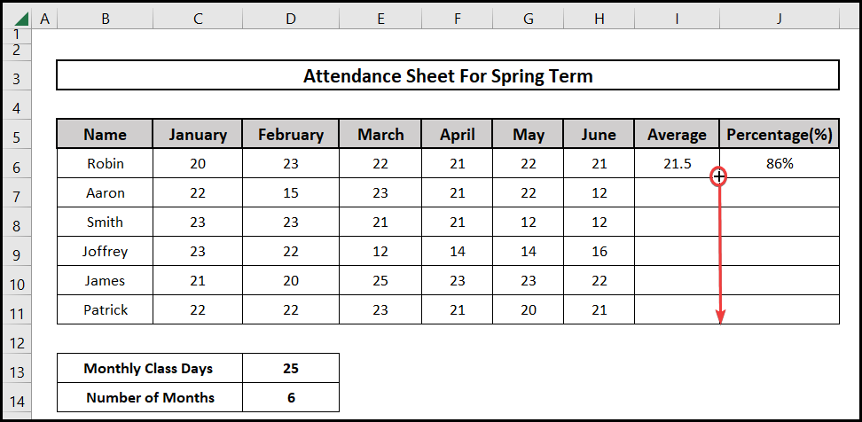
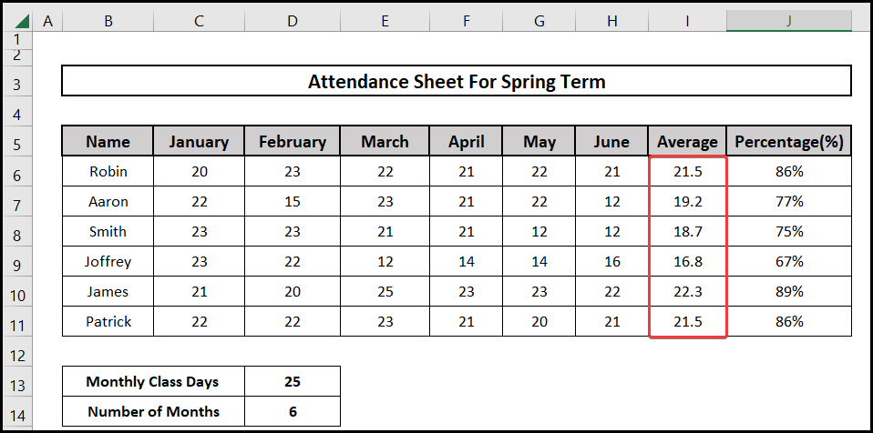
In this article, we will discuss 7 methods to prepare the average attendance formula in Excel. Let us assume that we have a dataset of the attendance for the Spring Term of an institution. We have the record from January to June. But now we are trying to calculate the Average Attendance of individual students. For our demonstration purpose, the sample data sheet along with the entries are given below.
1. Manual Calculation of Average Monthly Attendance with Formula
In this section, we will discuss how to Manually prepare the average attendance formula in Excel. This is the most simple process to determine the average. If we don’t want to use any Excel functions we can use this procedure. But the issue with this method is that if the data range is too large this method can become time-consuming. So the steps for using this method are as follows.
⬇️⬇️ STEPS ⬇️⬇️
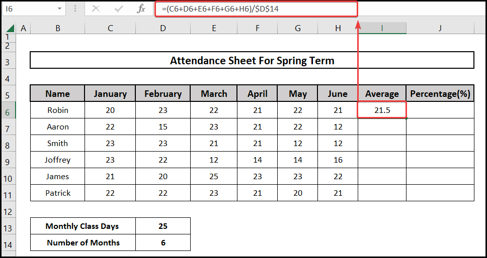
- Firstly we go to cell I6 and type this formula.
=(C6+D6+E6+F6+G6+H6)/$D$14
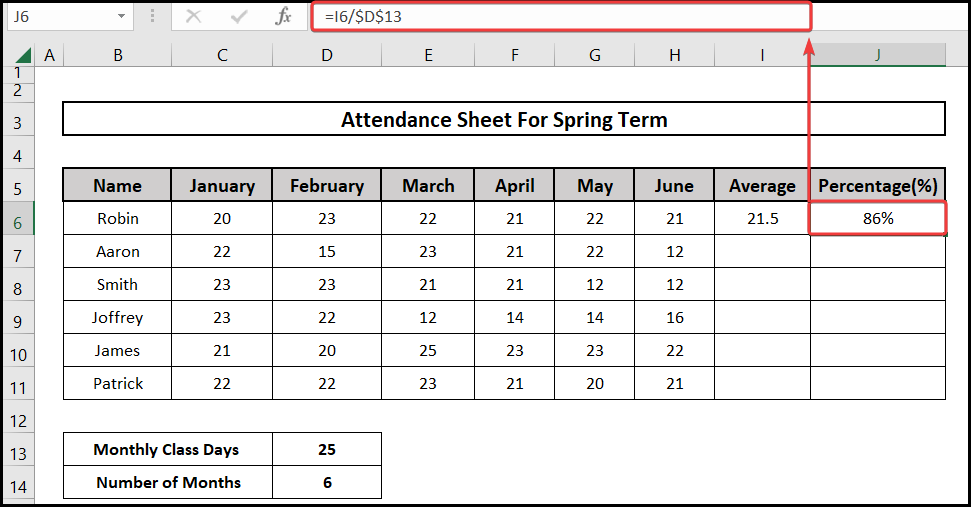
- We write this formula in cell J6 and determine the Percentage.
=I6/$D$13
- Following that we use the Fill Handle tool to drag the formula.
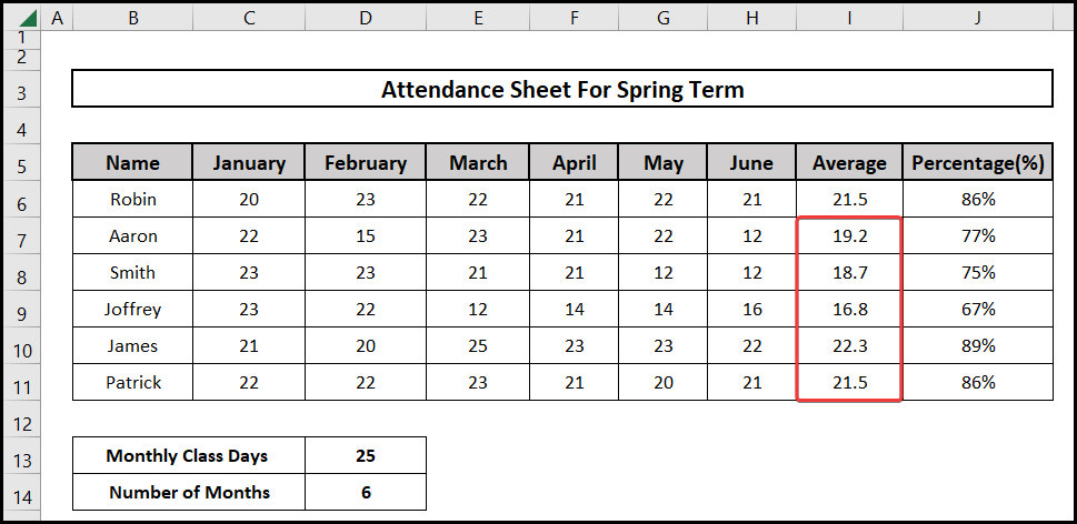
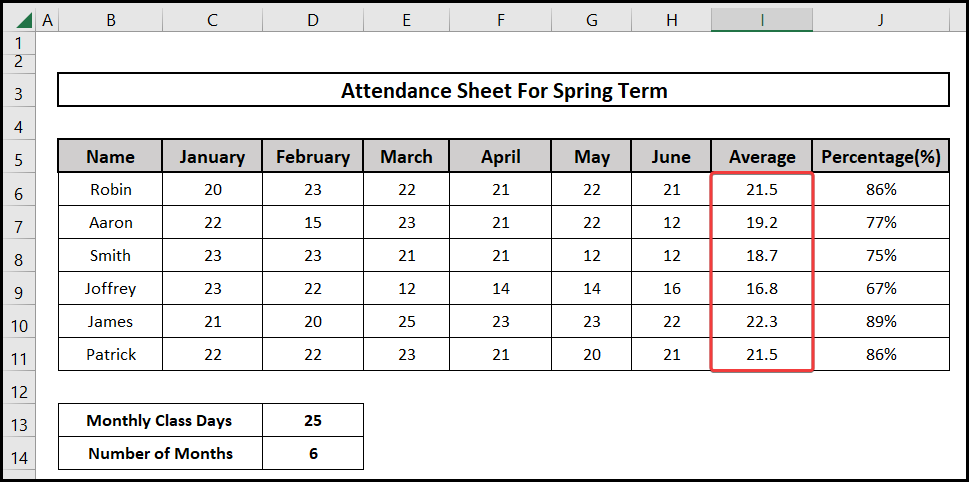
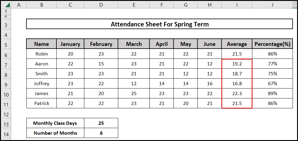
- Finally, we get the Average attendance in column I.
📕 Read More: 6 Quick Ways to Calculate Average Percentage of Marks in Excel
2. Applying AVERAGE Function
In this section, we will learn how we can use the AVERAGE function to prepare the average attendance formula in Excel. We can use this function to calculate the average of any given number range. So this is a very fast and accurate method. So the steps for using this method are as follows.
⬇️⬇️ STEPS ⬇️⬇️
- Firstly we go to the cell I6 formula box and write this formula.
=AVERAGE(C6:H6)
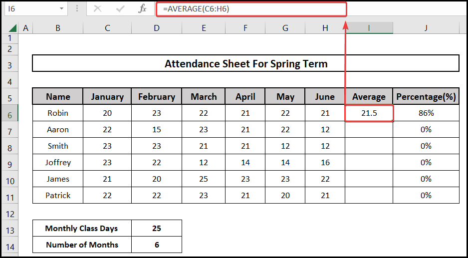
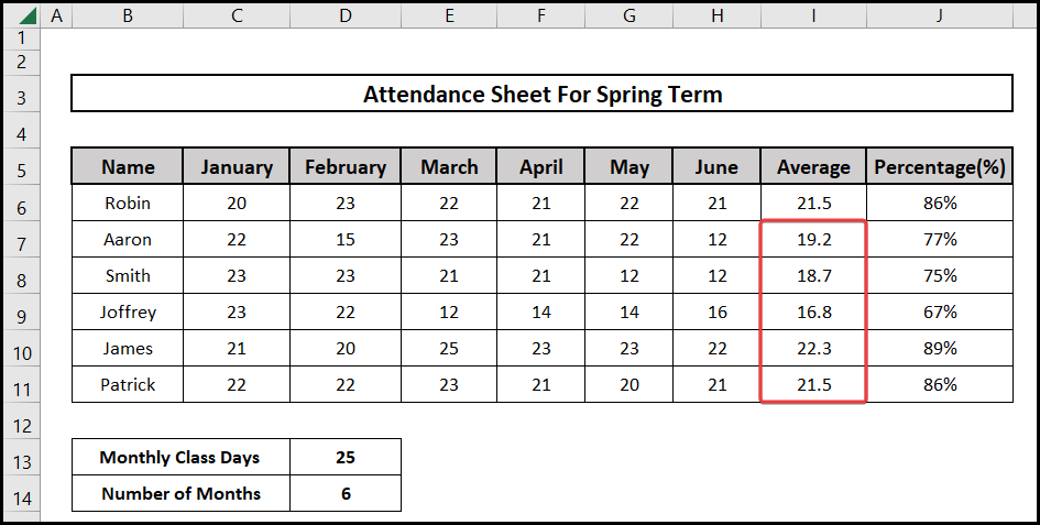
- After that, we use the Fill Handle tool to drag the formula.
- Finally, we get our result in column I.
📕 Read More: 7 Quick Ways to Calculate Average Percentage Increase in Excel
3. Utilizing AutoSum Feature
Here we will imply the Formula Tab from Ribbon to prepare the average attendance formula in Excel. This method is almost the same as the previous method. But the main difference is that here we use the Average function from the Formula Tab rather than writing ourselves. The steps for using this particular method are as follows.
⬇️⬇️ STEPS ⬇️⬇️
- Firstly we select the cells where we want the Average value.
- After that, we go to the Formulas Tab option.
- Following that we select the dropdown from the AutoSum option.
- Finally, we select the Average function.
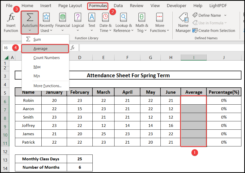
- We will immediately see the result in column I.
📕 Read More: How to Calculate Average Percentage Change in Excel
4. Applying Keyboard Shortcut to Calculate Average Attendance
In this section, we will learn how to use Keyboard Shortcuts to prepare the average attendance formula in Excel. This method is particularly beneficial if we don’t have any mouse available or have one that doesn’t respond properly. In that case, we can take the advantage of the Keyboard Shortcut. So the breakdown steps for this method are as follows.
⬇️⬇️ STEPS ⬇️⬇️
- Firstly we select the range where we want the Average value.
- Then we press these two keys together.
Alt+M
- Now we will see some shortcut keys on display.
- We press the U key.
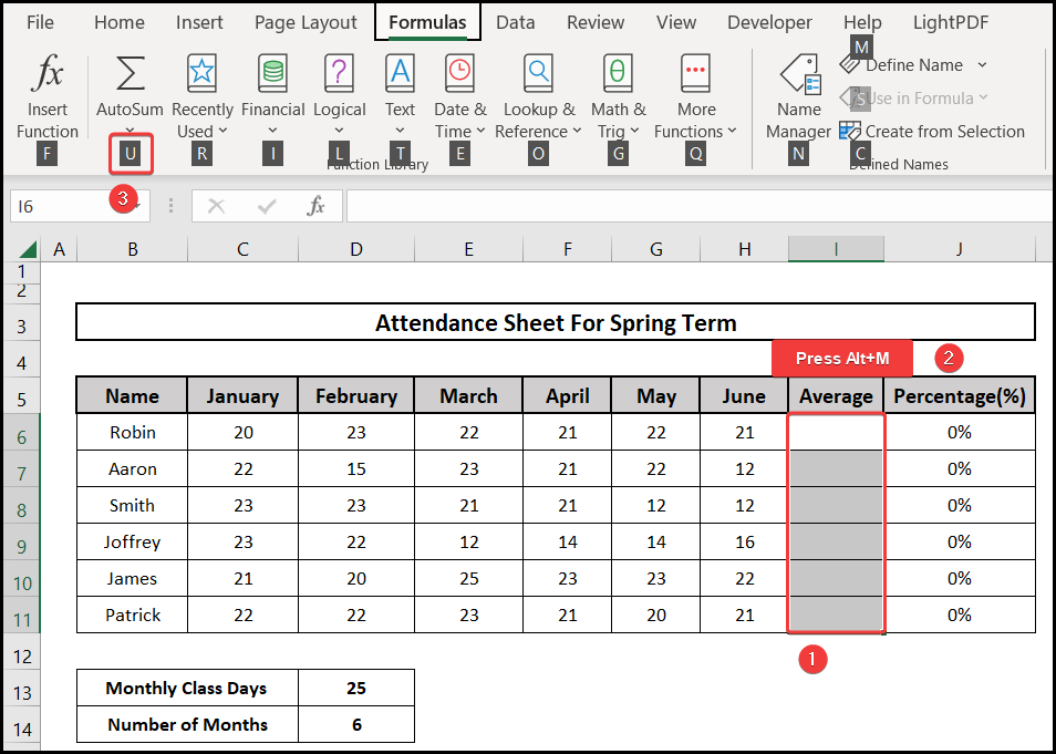
- After that, we press A from the keyboard to select the Average.
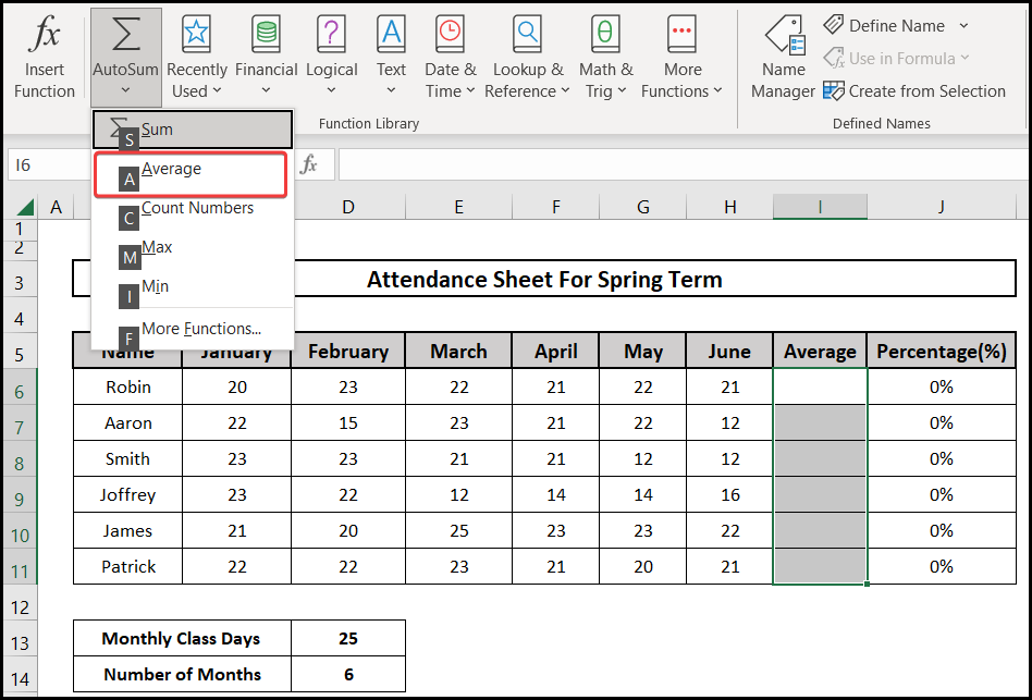
- Finally, we get the result in column I.
📕 Read More: 2 Easy Ways to Compute Average Excluding 0 in Excel
5. Implying SUMPRODUCT and SUM Functions Combined
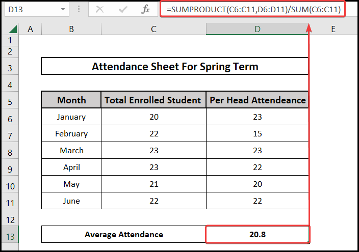
In this section, we will imply the SUMPRODUCT & SUM functions together to make the average attendance formula in Excel. This method is useful if we want to calculate the Weighted Average from some data set. Here we have the Total Enrolled Student & Per Head Attendance data. So we can easily determine the weighted average by this method. So the steps are as follows.
⬇️⬇️ STEPS ⬇️⬇️
- Firstly we go to the cell D13 formula box and write this formula.
=SUMPRODUCT(C6:C11,D6:D11)/SUM(C6:C11)
- Here SUMPRODUCT(C6:C11,D6:D11) returns us the summation of the product between columns C & D.
- We divide the value by the summation of column C to get the Average Attendance in cell D13.
📕 Read More: 6 Ways to Solve When Average Formula is Not Working in Excel
6. Using SUM & COUNT Functions Together
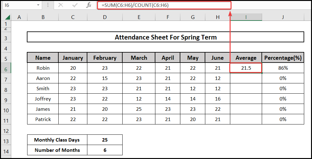
In this method, we will learn how to use the SUM & COUNT functions together to make the average attendance formula in Excel. This method uses two functions instead of one function like the previous method. But it is still a simple enough method and can also save us huge time. So the steps for using this method are as follows.
⬇️⬇️ STEPS ⬇️⬇️
- Firstly we go to the cell I6 formula box and type this formula.
=SUM(C6:H6)/COUNT(C6:H6)
- Here SUM(C6:H6) gives us the summation from the selected range.
- COUNT(C6:H6) returns the total cell number count from the range.
- Finally, we divide one by the other to get the Average.
- Following that we use the Fill handle tool to drag the formula.
- Finally, we get our result in column I.
📕 Read More: 7 Easy Ways to Calculate Average Rating in Excel
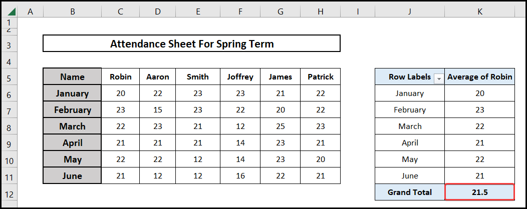
7. Using Pivot Table Feature
In our final section here we will use an Excel feature called Pivot Table to prepare the average attendance formula in Excel. Pivot Table is a very useful feature. It helps us to summarize data from a very large dataset. We can filter or add any data to a Pivot Table to make it more interactive. So to use this method we have to follow these steps.
⬇️⬇️ STEPS ⬇️⬇️
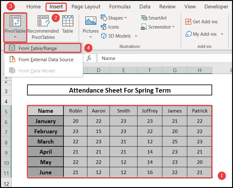
- Firstly we select our data range.
- After that, we go to the Insert tab.
- Following that we select the PivotTable option.
- Then we select the From Table/Range option.
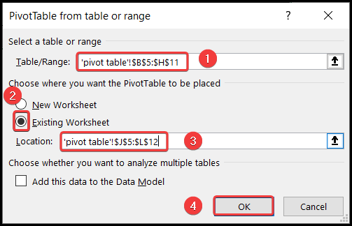
- Now we select the Range for Pivot Table.
- After that, we select the Existing Worksheet option.
- Following that we provide the Location where we want to create the Pivot Table.
- Then we select the OK button.
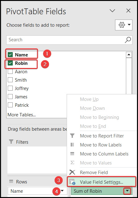
- Now we get a dialogue box named PivotTable Fields.
- After that we select the Name we want in our Pivot Table.
- Next, we go to the Value Field Settings.
- We select the Dropdown box as shown below.
- Now we select the Summarize value field by as Average.
- After that, we press the OK button.
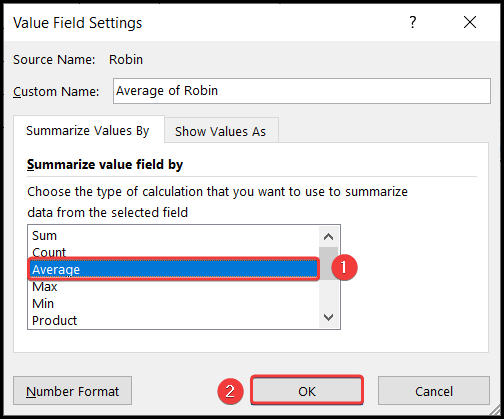
- Finally, we will see a Pivot Table right beside our data showing the Average in cell K12.
📄 Important Notes
🖊️ When we use Excel functions we have to be careful about function arguments.
🖊️ We have to be careful about case sensitivity when using the Keyboard Shortcuts.
📝 Takeaways from This Article
📌 We can Manually calculate the average attendance formula in Excel.
📌 We can utilize the AVERAGE function to prepare the average attendance formula in Excel.
📌 We can also use the Formula Tab from the Ribbon to prepare the average attendance formula in Excel.
📌 Keyboard Shortcut is another way to prepare the average attendance formula in Excel.
📌 Also we can imply the SUMPRODUCT function to do the same job.
📌 We can use the SUM & COUNT functions together to prepare the average attendance formula in Excel.
📌 Pivot Table is also an option to prepare the average attendance formula in Excel.
Conclusion
In this article, we have learned 7 different ways to calculate the average attendance formula in Excel. We can Manually calculate it, use the AVERAGE function, Utilize the Formula tab, apply Keyboard Shortcut, use functions like SUMPRODUCT or SUM & COUNT and use the Pivot Table feature to calculate the average attendance formula in Excel. Users can use any of the methods they feel comfortable with. If you want to ask any questions regarding this article you can put your question in the comment box. If you are looking for more Excel-related problems and solve processes you can visit our website www.Excelden.com.
Related Articles
- 3 Approaches to Calculate Average of Text in Excel
- 4 Approaches to Capitalize All Letters in Excel Without Formula
- 5 Ways to Calculate 7-Day Moving Average in Excel
- 3 Steps to Group Age Range in Excel Using VLOOKUP
- Calculate Displaced Moving Average with Formula in Excel


