While working with Excel, we might have to find the last row number with data. We can do that by applying different types of formulas. This article will briefly state about the methods by which we can find the last row number with data in Excel by using different types of formula.
📁 Download Excel File
Download the practice workbook below.
Learn to Find Last Row Number with Data Using Formula in Excel with These 2 Suitable Approaches
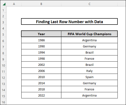
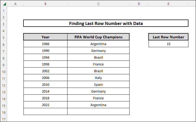
To demonstrate things easily, we will consider a dataset where the FIFA World Cup winners across different years from 1986 to 2022 are presented in a table. We will use this table to find out the last row number with data for both non-blank cells and combination of blank and non-blank cells. The sample dataset is shown as follows:
1. For Non-Blank Cells
In this approach, we will be counting the last row number for non-blank cells. That is, within the dataset range, there will be no blank cells. There are two ways of finding the last row number by this approach. These are as follows:
1.1 Incorporating MIN, ROW and ROWS Functions
The functions MIN, ROW, and ROWS can be combined to generate a formula. Using this formula, we can find the last row number in a dataset. The steps for this approach are as follows:
⬇️⬇️ STEPS ⬇️⬇️
- In the beginning, we select cell E6.
- After that, we move over to the formula bar and write the following formula and press Enter.
=MIN(ROW(B6:C15))+ROWS(B6:C15)-1🔨 Formula Breakdown
MIN(ROW(B6:C15))+ROWS(B6:C15)-1
👉 ROWS function gives an output of the number of rows present in the range B6:C15.
👉 ROW function gives an output of the row number of a reference used as an argument.
👉 MIN function delivers the minimum value in a certain range of data.
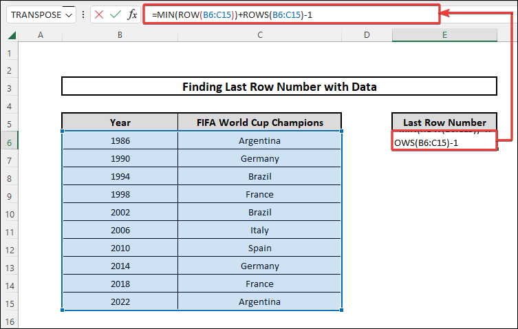
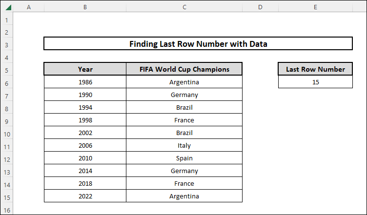
- Thus, we will get the row number of the last row where data is present within the cell range.

1.2 Using ROW, INDEX and ROWS Functions
In this approach, we will be incorporating ROW, INDEX, and ROWS functions to put together a formula to find the last row number with data in Excel. The steps for this approach are as follows:
⬇️⬇️ STEPS ⬇️⬇️
- At first, we select cell E6.
- After that, we go to the formula bar and write the following formula, and press Enter.
=ROW(INDEX(B6:C15,1,1))+ROWS(B6:C15)-1🔨 Formula Breakdown
ROW(INDEX(B6:C15,1,1))+ROWS(B6:C15)-1
👉 ROWS function gives an output of the number of rows present in the range B6:C15.
👉 INDEX function gives the output value of the cell where the second argument 1 is the row number and the second argument 1 is the column number. B6:C15 is the range of cells from which the rows and columns are to be counted.
👉 ROW function gives an output of the row number of a reference used as an argument.
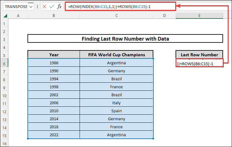
- As a result, the output that we will get will have the row number of the last row where data is present within the cell range.
 Read More: 4 Quick Ways to Find Last Column with Data in Excel
2. For Both Blank and Non-Blank Cells
In this approach, we will be counting the last row number for both blank and non-blank cells present. That is, within the dataset range, there will be both blank and non-blank cells. But the formulas will identify the last non-empty row and give the output as such. There are five ways of finding the last row number by this approach. These are as follows:
2.1 Using MATCH and REPT Functions
The process of using MATCH and REPT functions to find the last row number consisting of blank and non blank cells are as follows:
⬇️⬇️ STEPS ⬇️⬇️
- We select the cell E6 and write down the following formula in the formula bar.
=MATCH(REPT("z",50),C:C)🔨 Formula Breakdown
MATCH(REPT(“z”,50),C:C)
👉 REPT function repeats a text where the first argument is the text we intend to repeat and the second argument specifies how many times we want to repeat it. Here z is repeated 50 times.
👉 MATCH function has three arguments. The first argument is the value we want to look up, the second argument denotes where we want to look the value, in this case, the column C.
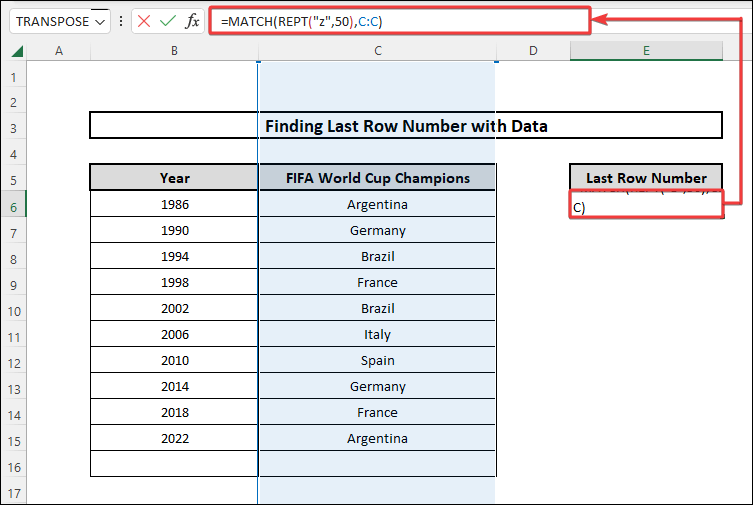
- After that, we press Enter.
- We will see that the output of the last row number reveals as 15. Here although the table has one blank cell, the output comes out counting the last row as the cell that has some value.

2.2 Applying MAX Function
The MAX function gives the largest value as output from a set of data. This function can find the last row number in a dataset by the following steps:
⬇️⬇️ STEPS ⬇️⬇️
- At first, we select the cell E6.
- Next, we hover over to the formula bar and write the following formula and press Enter.
=MAX((B:B<>"")*(ROW(B:B)))🔨 Formula Breakdown
MAX((B:B<>””)*(ROW(B:B)))
👉 ROW function gives an output of the row number of a reference used as an argument and in this case, it is all cells within column B.
👉 MAX function gives the maximum value from a set of numbers.
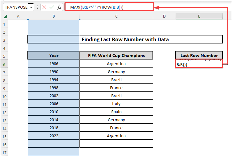
- Therefore, we will get the row number of the last row where data is present within the cell range. The output we will receive is the digit 15, where 15 is the last row number that has a value.
2.3 Inserting SUMPRODUCT Function
SUMPRODUCT function gives an output of the sum of the products of related ranges or arrays. This function can help find the last row number with data along with MAX and ROW function. The steps in this approach are as follows:
⬇️⬇️ STEPS ⬇️⬇️
- Like the previously mentioned approaches, at first, we select a definite cell E6.
- Then, we write the following formula in the formula tab on the top.
=SUMPRODUCT(MAX((C5:C16<>"")*ROW(C5:C16)))🔨 Formula Breakdown
SUMPRODUCT(MAX((C5:C16<>””)*ROW(C5:C16)))
👉 ROW function gives an output of the row number of a reference used as an argument. Here the argument inside C5:C16 gives an output of the number of rows.
👉 MAX function gives the maximum value from a set of numbers.
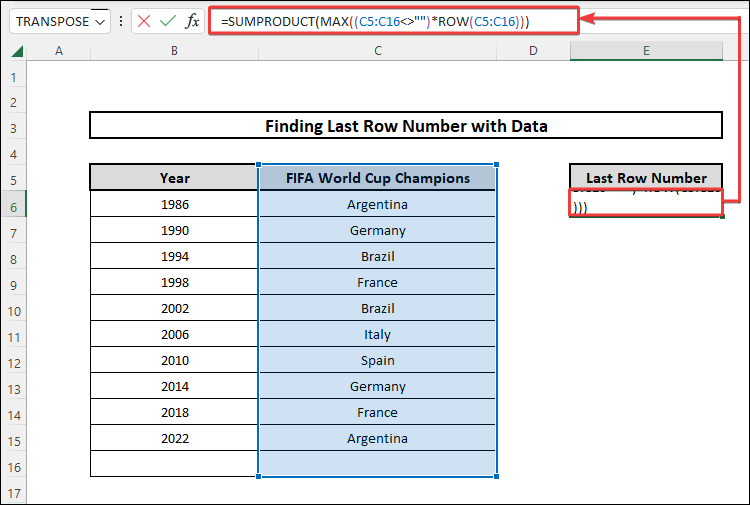
- After that, we press Enter.
- The output result will show that the last row number is 15, despite having a blank cell just below row 15.

2.4 Utilizing LOOKUP Function
The LOOKUP Formula in Excel is used to look up a value within one column range or one-row range. This function is widely used to find certain values within a dataset. The steps of using this approach are as follows:
⬇️⬇️ STEPS ⬇️⬇️
- First, we select cell E6.
- After that, we go to the formula tab and write down the following formula.
=LOOKUP(2,1/(B:B<>""),ROW(B:B))🔨 Formula Breakdown
LOOKUP(2,1/(B:B<>””),ROW(B:B))
👉 ROW(B:B) indicates the number references of the column B.
👉 LOOKUP function looks for a value specified in the first argument, the second row indicate the row or column range where we need to search.
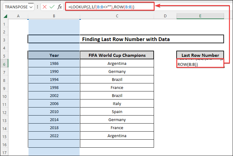
- Then we press Enter.
- The results will reveal similar to the following image.

Read More: 5 Ways to Find First Occurrence of a Value in a Range in Excel
How to Find Last Row Number with Data Using Excel VBA
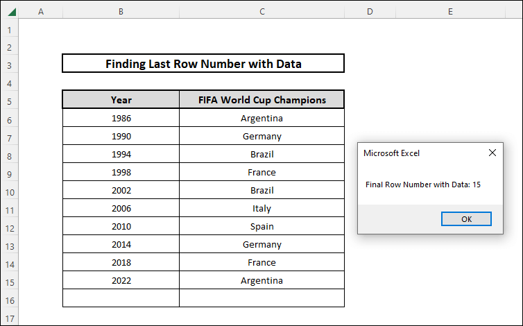
We can use VBA Code to find out the last non-blank row number. In the dataset we will use for this method, there is one blank row at the end. The steps for writing a VBA code are as follows:
⬇️⬇️ STEPS ⬇️⬇️
- In the beginning, we go the sheet where we will be showing this VBA code approach.
- We right-click on the VBA Code sheet and select View Code.
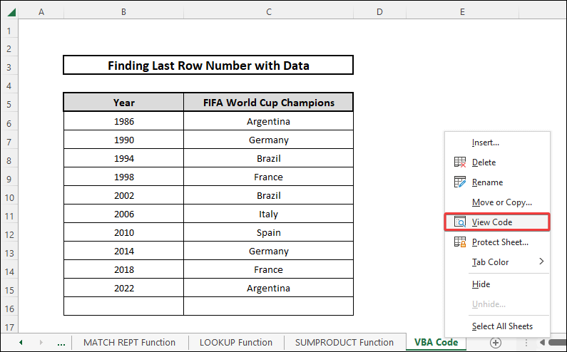
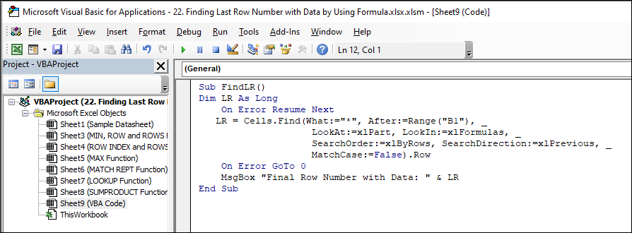
- A new window will appear. We write the following VBA code on that window.
Sub FindLR()
Dim LR As Long
On Error Resume Next
LR = Cells.Find(What:="*", After:=Range("B1"), _
LookAt:=xlPart, LookIn:=xlFormulas, _
SearchOrder:=xlByRows, SearchDirection:=xlPrevious, _
MatchCase:=False).Row
On Error GoTo 0
MsgBox "Final Row Number with Data: " & LR
End Sub- Then we press Run or alternately, the shortcut key F5.
- A pop-up message box will appear showing the last row number like the following image.
📄 Important Notes
🖊️ The REPT function does not work on numbers. So, while using the function to find the last row number, we must be careful so that the selected range does not contain numerical data.
🖊️ LOOKUP function will match the next smallest value if lookup value cannot be found.
🖊️ SUMPRODUCT function considers the non-numeric items as zeros.
📝 Takeaways from This Article
You have taken the following summed-up inputs from the article:
📌 To find the last row number with data where no blank cells are present in the dataset, we can use a combination of MIN, ROW, ROWS, and INDEX functions.
📌 For both blank and non-blank cells, we can use multiple functions such as MATCH, REPT, MAX, SUMPRODUCT, and LOOKUP functions.
📌 Alternatively, a VBA Code can also help us to find the last row number with data with blank and non-blank cells in a dataset.
Conclusion
In conclusion, I hope that this article has provided you with insights about how we can find the last row number from a range of data in Excel. If you want to know more about Excel, please visit our site ExcelDen and if you have any queries regarding this topic, feel free to let us know down below in the comment section.
Related Articles
- 5 Ways to Return True If Value Exists in Column in Excel
- 3 Ways to Check If Range of Cells Contains Specific Text in Excel


