Excel VBA: If Font Color Is Red Then Return Specific Output

We can return different types of output if the font color is red in certain cells in Excel. This article will discuss the ways in which we can return a specific output if font color is red in Excel.

Contents hide

📁 Download Practice Workbook

Learn to Return Specific Output If Font Color Is Red in Excel with These 6 Suitable Approaches

1. Returning Index Number If Font Color Is Red

2. Providing Text If Font Color Is Red

3. Highlighting Cells If Font Color Is Red

4. Getting Font Color Code If Font Color Is Red

5. Changing Font Color If Font Color Is Red

6. Providing RGB Code If Font Color Is Red

📄 Important Notes

📝 Takeaways from This Article

Conclusion

📁 Download Practice Workbook

Download the practice workbook below.

Return Specific Output If Font Color Is Red.xlsm

Learn to Return Specific Output If Font Color Is Red in Excel with These 6 Suitable Approaches

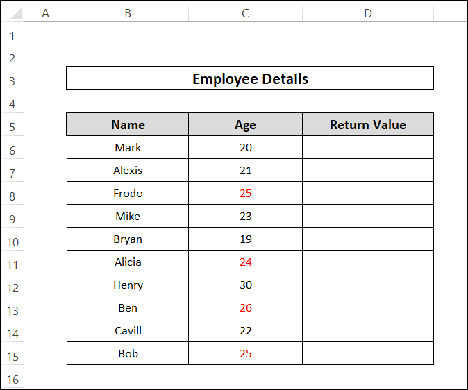
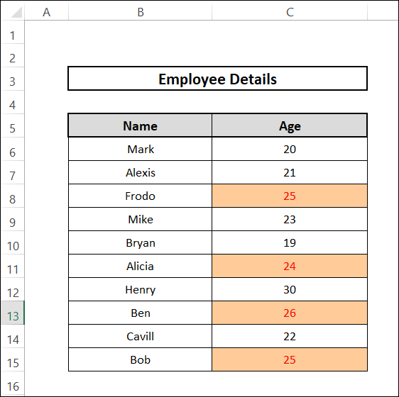
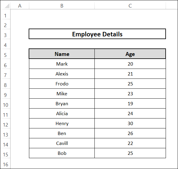
To demonstrate things easily, we will consider a dataset where we have the names and ages of different people and within this dataset, we have some ages marked in red. We also have a column with the name Return value. We will use this column to get an output of the cells that have their font color in red. The dataset is as follows:

Example

1. Returning Index Number If Font Color Is Red

In this approach, we will get an output of Index number on the instances where the font color is red. The steps for this approach are as follows:

⬇️⬇️ STEPS ⬇️⬇️

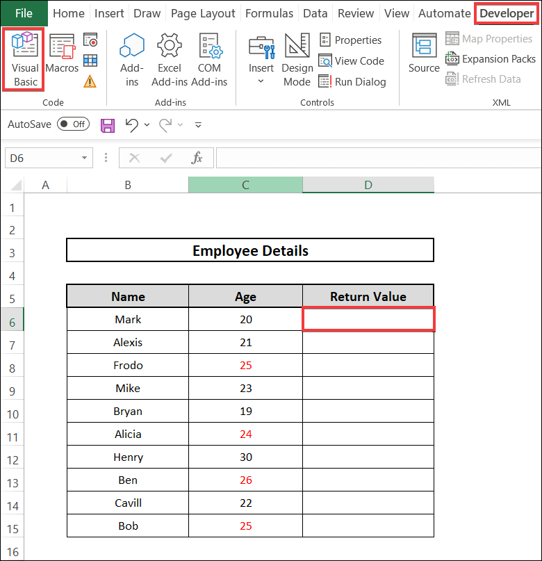
At first, we click Alt+F11 to go to Visual Basic Editor. Alternatively, we can go to Developer options and select Visual Basic.

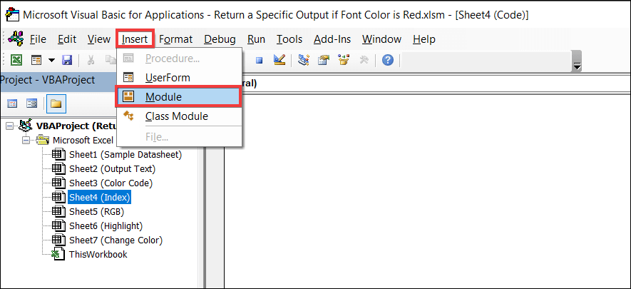
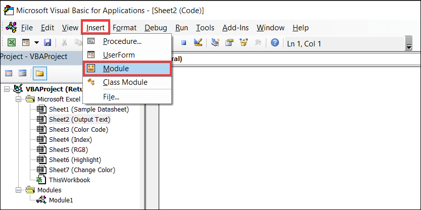
Then we click on Insert and select a new Module.

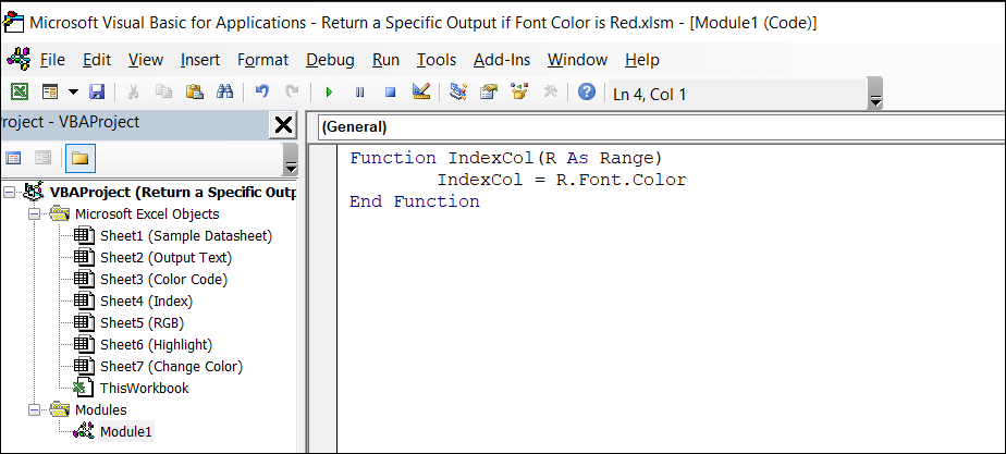
After creating the new module, we write the following VBA Code in the window.

Function IndexCol(R As Range)
IndexCol = R.Font.Color
End Function

After that, we close the module window and go to the cell D6.
We select the cell D6 and call the user defined function as stated in the VBA Code named IndexCol().
We write the following formula in the formula bar.

=IndexCol(C6)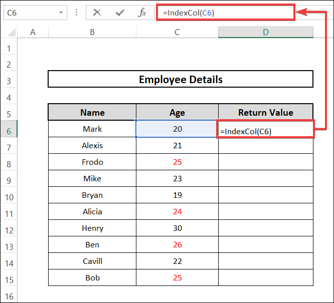

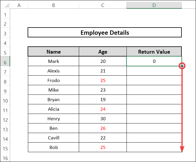
Then, we drag the Fill Handle on the bottom right of the cell D6 and drag it all the way up to cell D15.

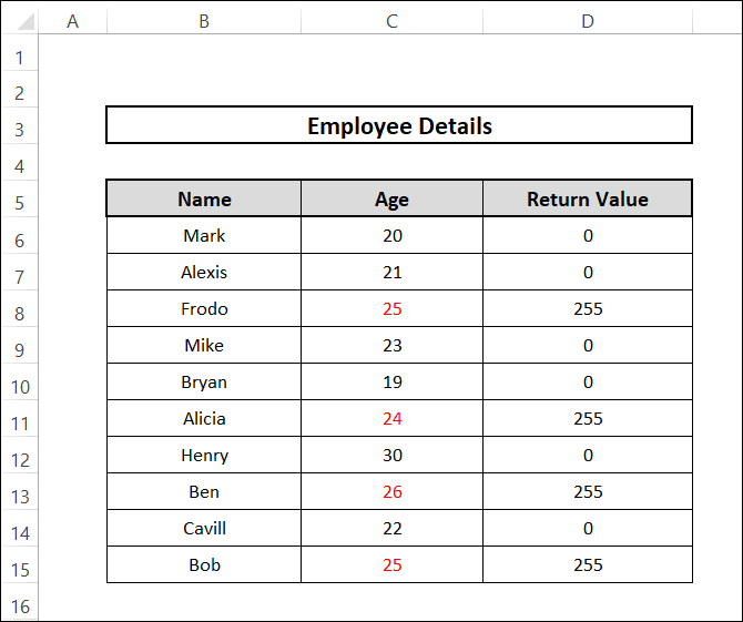
The index numbers of cells with red color font will show up as having an index number value of 255 like the following image.

Example

2. Providing Text If Font Color Is Red

In this approach, we will be getting a text as an output if the font color is red. To state specifically, we will be getting a text output of whether the font color is red or not. To do this, we need to follow these steps.

⬇️⬇️ STEPS ⬇️⬇️

At first, we press Alt+F11 and go to the Editor named Visual Basic.
Then, we click on Insert and then select Module to create a new one.

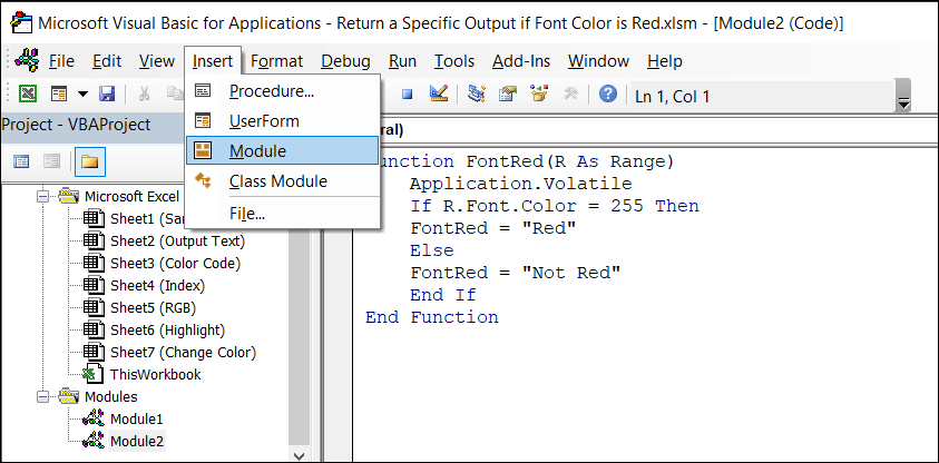
In the new module, we write the following VBA Code.

Function FontRed(R As Range)
 Application.Volatile
 If R.Font.Color = 255 Then
 FontRed = "Red"
 Else
 FontRed = "Not Red"
 End If
End Function

Then we close the window and call the stated function in the code named FontRed()
We write the following formula in the formula bar.

=FontRed(C6)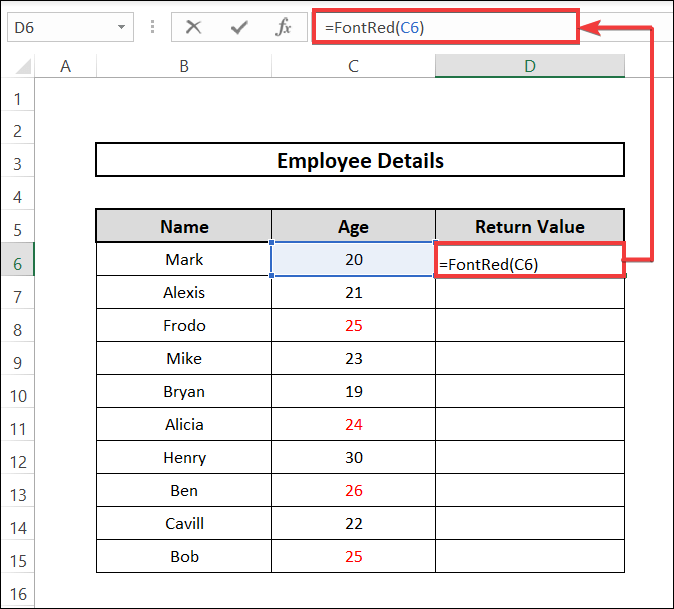

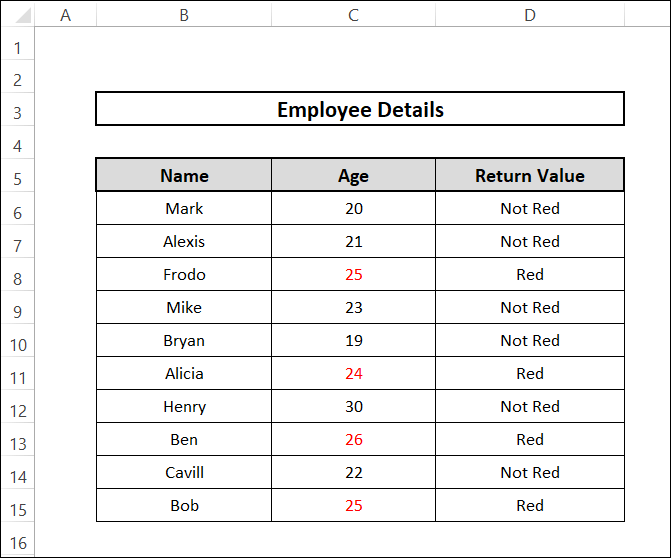
After that, we drag the Fill Handle of cell D6 and drag it up to the cell D15.

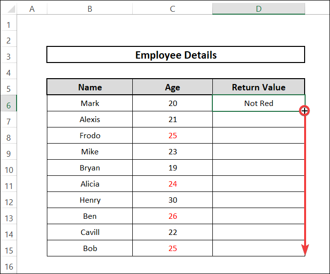
The results will be like the following image.

Example

3. Highlighting Cells If Font Color Is Red

Suppose we are aiming to highlight cells which have numbers written in red color font. To do so, we need to do follow these steps.

⬇️⬇️ STEPS ⬇️⬇️

Firstly, we press Alt+F11 and go to the Editor named Visual Basic.
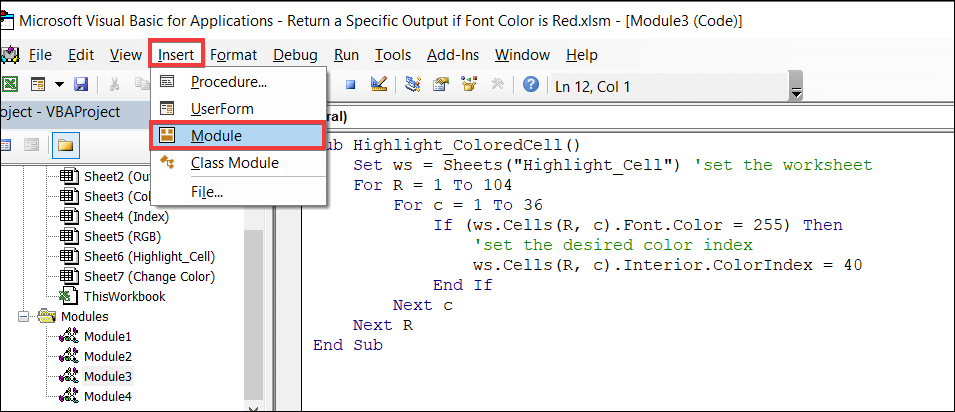
After that, we click on Insert and then select Module to create a new one.

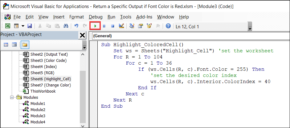
In the new module, we write the following VBA Code.

Sub Highlight_ColoredCell()
Set ws = Sheets("Highlight_Cell") 'set the worksheet
For R = 1 To 104
For c = 1 To 36
If (ws.Cells(R, c).Font.Color = 255) Then
ws.Cells(R, c).Interior.ColorIndex = 40
End If
Next c
Next R
End Sub

Then we run the code by clicking on the Run.

The results will be like the following image where the red colored font cells will be highlighted.

Example

4. Getting Font Color Code If Font Color Is Red

To get the font color code for cells having red-colored texts or numbers present in them, we can follow the following steps.

⬇️⬇️ STEPS ⬇️⬇️

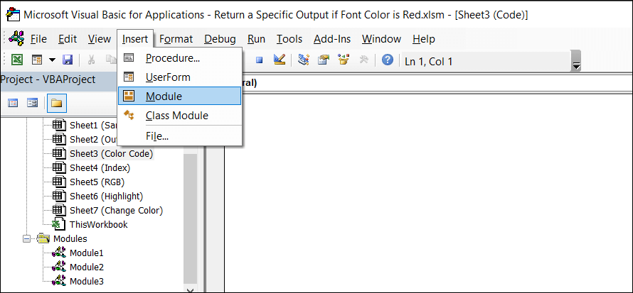
At the beginning, we press Alt+F11 and go to the Visual Basic Editor.
After that, we click on Insert and then select Module to create a new module.

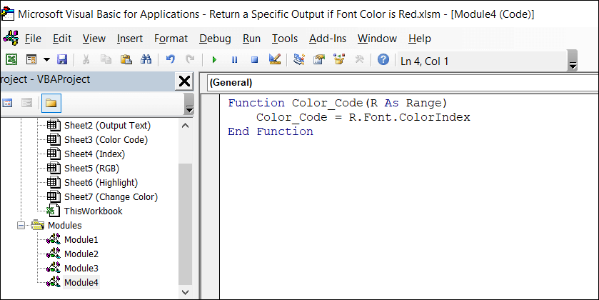
In the new module, we write the following VBA Code.

Function Color_Code(R As Range)
Color_Code = R.Font.ColorIndex
End Function

Then we close the window and call the stated function in the code-named Color_Code()
We write the following formula in the formula bar.

=Color_Code(C6)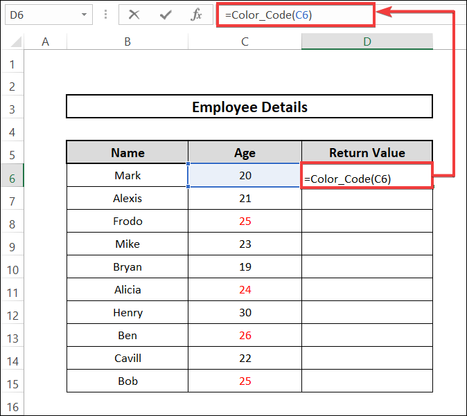

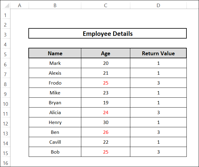
After that, we drag the Fill Handle of cell D6 and drag it up to the cell D15.

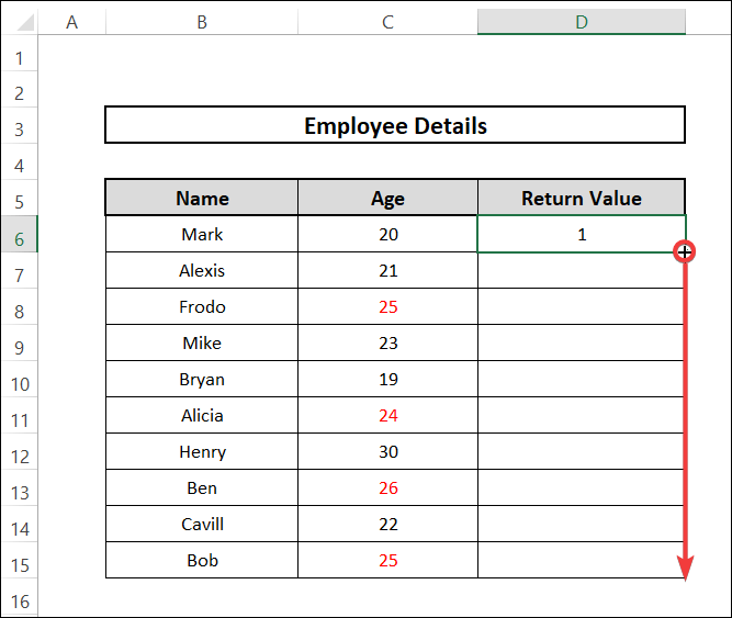
The results will be visible in the following image.

Example

5. Changing Font Color If Font Color Is Red

In this approach, we will change font color to black from red for the cells that have entries in red color font. To do so, we need to follow these steps.

⬇️⬇️ STEPS ⬇️⬇️

As the first step, we press Alt+F11 and go to Visual Basic.
After that, we click on Insert and then select Module to create a new one.

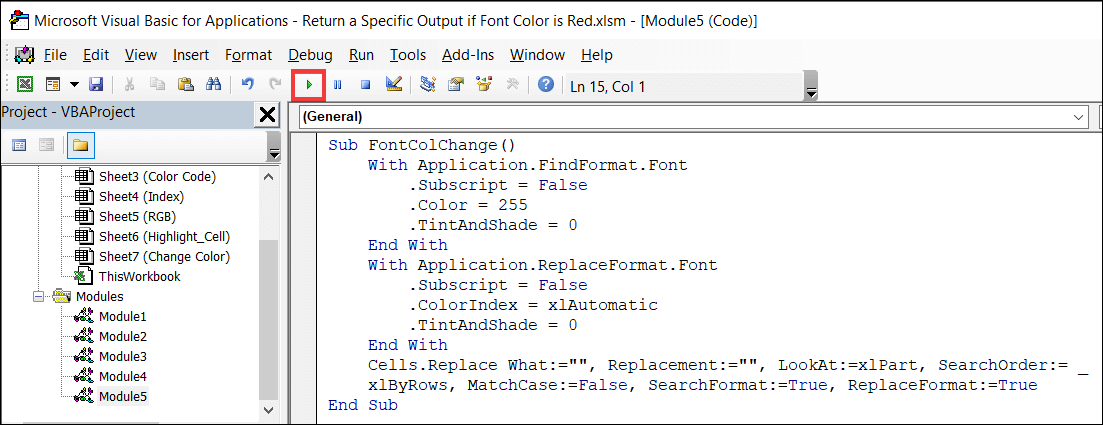
In the new module, we write the following VBA Code.

Sub FontColChange()
With Application.FindFormat.Font
.Subscript = False
.Color = 255
.TintAndShade = 0
End With
With Application.ReplaceFormat.Font
.Subscript = False
.ColorIndex = xlAutomatic
.TintAndShade = 0
End With
Cells.Replace What:="", Replacement:="", LookAt:=xlPart, SearchOrder:= _
xlByRows, MatchCase:=False, SearchFormat:=True, ReplaceFormat:=True
End Sub

We press the Run button after writing the code.

The results will be visible in the following image.

Example

6. Providing RGB Code If Font Color Is Red

In this approach, we will be obtaining the RGB Code as output for the red-colored entries. We can do this by following these steps.

⬇️⬇️ STEPS ⬇️⬇️

At first, we press Alt+F11 and go to the Visual Basic Editor.
After that, we click on Insert and then select Module to create a new module.

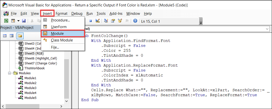
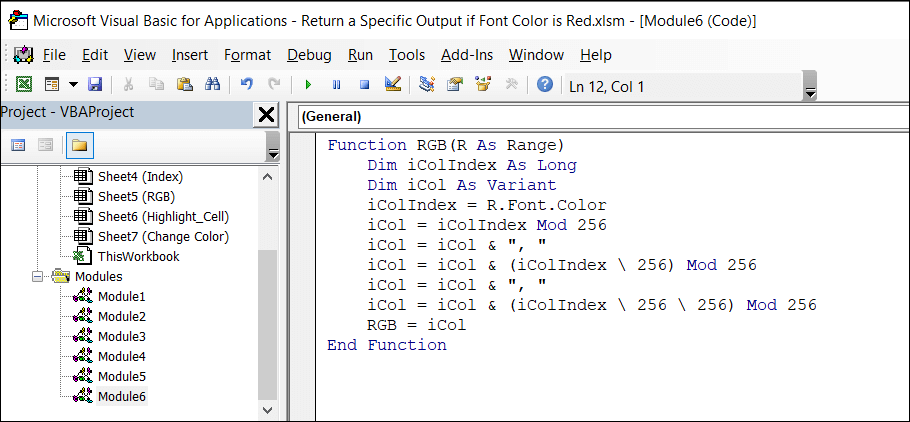
In the new module, we write the following VBA Code.

Function RGB(R As Range)
 Dim iColIndex As Long
 Dim iCol As Variant
 iColIndex = R.Font.Color
 iCol = iColIndex Mod 256
 iCol = iCol & ", "
 iCol = iCol & (iColIndex \ 256) Mod 256
 iCol = iCol & ", "
 iCol = iCol & (iColIndex \ 256 \ 256) Mod 256
 RGB = iCol
End Function

Then we close the window and call the stated function in the code-named RGB()
We write the following formula in the formula bar.

=RGB(C6)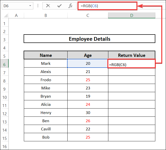

After that, we drag the Fill Handle of cell D6 and drag it up to cell D15.

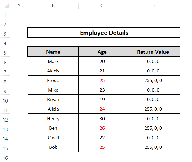
The output results will look like the following image.

📄 Important Notes

🖊️ If the Developer tab is not visible then we enable it by selecting Customize Ribbon from Options in the File tab. Then we check the Developer box under the Main Tabs option in the Customize the Ribbon section.

🖊️ For user-defined functions, we don’t have to run the VBA Code. We can just save it and call the function later.

🖊️ If the Macro Enabled workbook xlsm cannot be opened or viewed, then we can enable it by selecting Enable all macros in the Macro settings under Trust Center Settings that can be found in the options menu of the File tab.

📝 Takeaways from This Article

You have taken the following summed-up inputs from the article:

📌 We can get the Index number, Output Text, Color Code value and RGB Code as output for cells that have red-colored entries by creating user-defined functions with the help of VBA Code.

📌 We can also write VBA Code and run them for highlighting cells and change the color of cells that have red font-colored entries.

Conclusion

In conclusion, I hope that this discussion has provided you with insights into how we can return a specific output when the font color is red in Excel. If you want to know more about Excel, please visit our site ExcelDen and if there is any query regarding this topic, feel free to let us know down below in the comment section.