5 Ways to Insert Dynamic Sheet Name in Excel Formula

Sometimes we need to use data from different sheets. In this case for a small dataset, we do a hectic job like copying and pasting the data to a new workbook/sheet. But what we can do to get rid of these issues is, to use sheet name in the dynamic formula in Excel. In this article, learn to use sheet name in formula dynamic, we will discuss several methods to use sheet names in dynamic formulas.

📁 Download Excel File

To practice please download the excel file from here:

Learn to Insert Dynamic Sheet Name in Excel Formula with 5 Ways

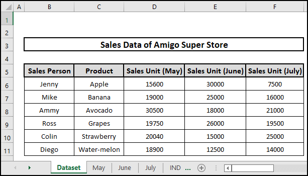
We consider a dataset named Sales Data of Amigo Super Store. In the dataset, there is 5 heading containing Sales Person, Product, Sales Unit(May), Sales Unit(June), and Sales Unit(July). There are also 6 columns as well as 11 rows in the dataset. In this article, we are going to use INDIRECT, VLOOKUP, INDEX, and HYPERLINK functions.

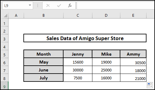
We also have 3 separate datasets for each month May, June, and July containing 4 columns and 11 rows.

Using the INDIRECT function you can insert data from any sheet of the same workbook. Please follow the below steps.

 ⬇️⬇️ STEPS ⬇️⬇️

• First, select a blank cell i.e. C6.
• Secondly, Insert the following formula in C6 containing the INDIRECT function.

• Therefore, we get the value at D6.

• Auto-filling we finally get the total output for Jenny, Mike, and Ammy.

Using the VLOOKUP function to look up the values in another sheet can be another way to link and get values. Please follow the necessary procedure.

 ⬇️⬇️ STEPS ⬇️⬇️

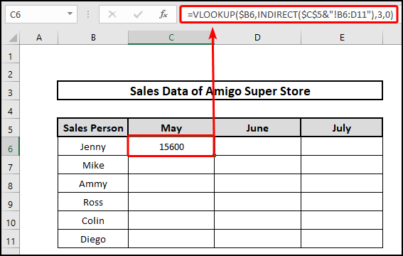
• Initially navigate a blank cell i.e. C6.
• Secondly, Insert the following formula in C6 containing the INDIRECT and VLOOKUP functions.

• Finally, we obtain the sales data for Jenny in May from sheet May.

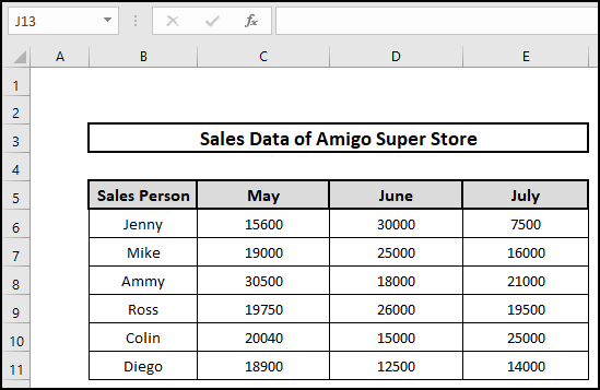
• Using Fill Handle or Auto-filling the table, we similarly obtain all the data in a separate sheet.

With an index column, and calling sheet names using INDEX and HYPERLINK functions, you can easily jump any worksheet in a workbook very easily. Please check out the steps below.

 ⬇️⬇️ STEPS ⬇️⬇️

• Initially make an Index.
• Then from Formulas Menu, select Define Name.

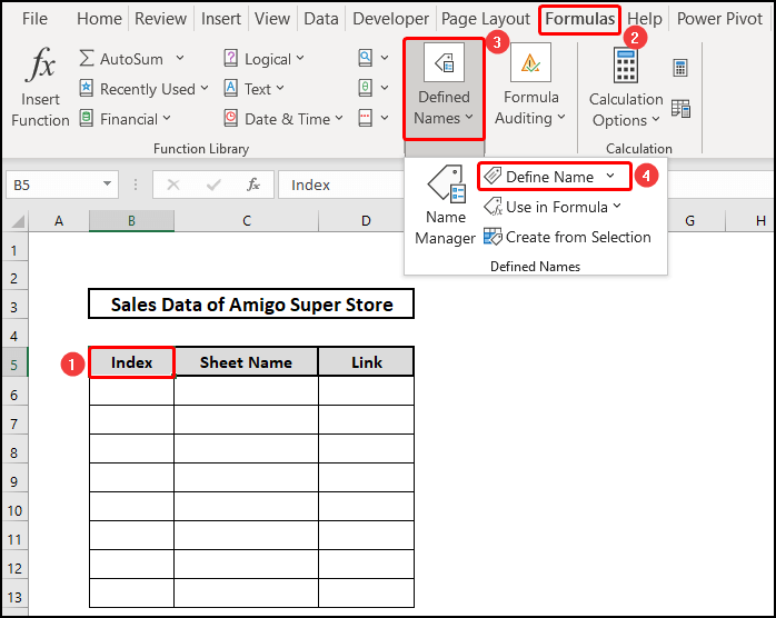
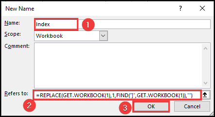
• A box named New Name appears.
• Type the Name and insert the following formula in Refers to.

• Then click on the OK button.

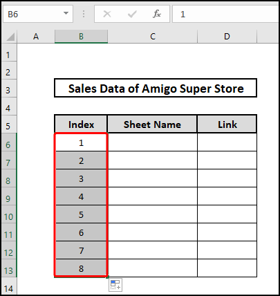
• Now write the index number in ascending order (1,2,3…) under the Index column.

• Next, insert the following formula in C6.

• The INDEX function finds the sheet name using B6 accordingly and the sheet name is Dataset.

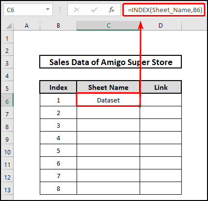
• Finally, using Fill Handle, we obtain sheet names in the Sheet Name column.

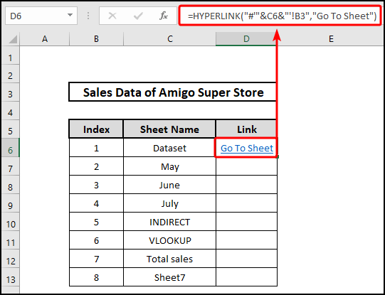
• Again in D6, insert the following formula containing HYPERLINK to jump into the sheet.

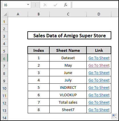
• Now, by clicking on Go To Sheet, we can go to the sheet Dataset.
• Auto-filling the column, we get the desired output containing hyperlinks.
• Finally, we can jump to any sheet by clicking on the cell.

We can use the VBA code to get the sheet name from a cell value. With the help of the Developer option, you can generate a program of your own. Please follow the steps.

⬇️⬇️ STEPS ⬇️⬇️

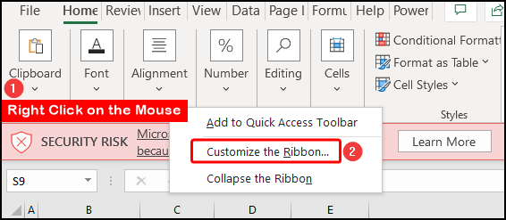
• First, Check if your Developer option is available or not.
• Then to enable the Developer option, right-click on the mouse at the top Ribbon and select Customize the Ribbon.

• Click on Developer and click on OK.

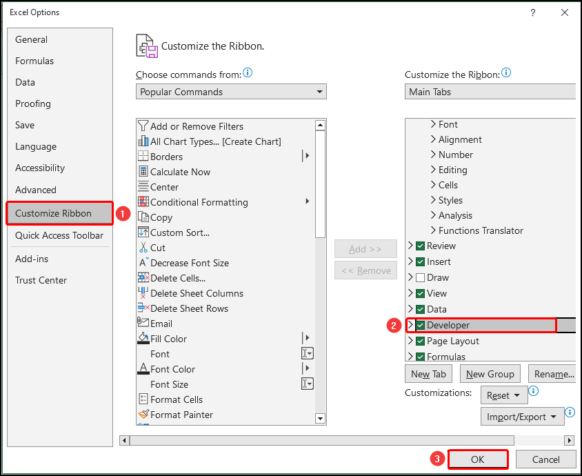
• Now Developer mode is on.
• Click on the Visual Basic option.
• To insert the VBA code, click on Module from the Insert option.

• Insert the following code in the Module and click Run to execute the VBA Macro.

Code:

Private Sub Worksheet_SelectionChange(ByVal Target As Range)
Set Target = Range("C5")
If Target = "" Then Exit Sub
Application.ActiveSheet.Name = VBA.Left(Target, 31)
Exit Sub
End Sub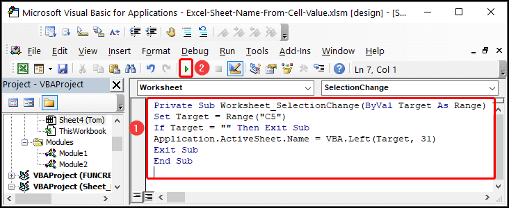

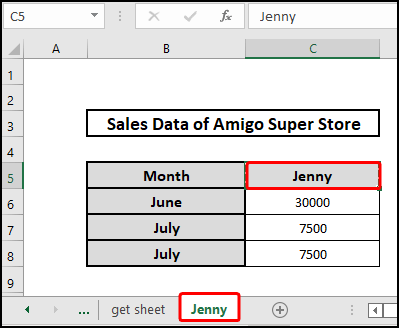
• Therefore, we get the Sheet name Jenny from cell C5.

Suppose you need to prepare a workbook only to count total sales from another workbook. What to do? Let’s follow the procedure to get data from another workbook.

⬇️⬇️ STEPS ⬇️⬇️

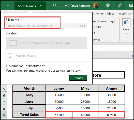
• First, Open the workbook from where you want to import data.
• Secondly, Inspect the File name and Sheet name very carefully.
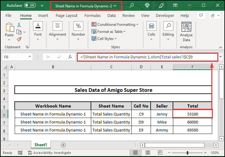
• Then, select a cell i.e. F6, and insert the following formula.

• Formula ='[Sheet Name in Formula Dynamic 1.xlsm]Total sales’!$C$9 denotes to open sheet Total sales from Excel file Sheet Name in Formula Dynamic 1.xlsm and take value from $C$9.

• Therefore, in the new workbook, we get our output from another workbook named Sheet Name in Formula Dynamic-1.

📄 Important Notes

🖊️  Be careful and measure accurately during working with different sheets and workbooks. Otherwise, you will lose your data.

🖊️  Don’t close workbooks while working with multiple workbooks and sheets.

🖊️  During working with VBA code, check whether your Developer tool is available.

📝 Takeaway from This Article

📌  INDEX function to get Sheet Names from the same workbook.

📌  VLOOKUP and INDIRECT functions to get the data from different sheets.

📌  HYPERLINK function to jump to a particular sheet.

📌  Linking Workbooks to one another to make them dynamic.

📌  VBA to make sheet name from cell value.

Conclusion

We demonstrated every possible use of sheet names in the dynamic formulas in Excel. I hope you enjoyed your learning. Any suggestions as well as queries appreciated. For better understanding and new knowledge don’t forget to visit www.ExcelDen.com.

Related Articles

• Pull Same Cell from Multiple Sheets into Master Column
• Difference Between Absolute and Relative Reference in Excel