5 Ways to Add Gridlines After Highlighting in Excel

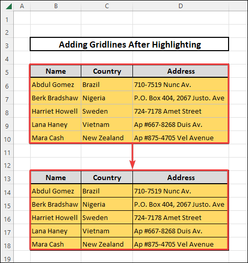
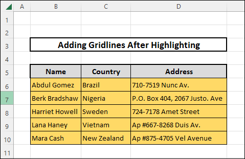
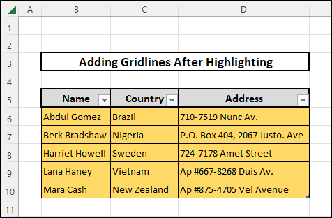
Gridlines are the horizontal and vertical lines that are present among cells in Excel. These gridlines help us to navigate the position of each cell and separate our data entries. When we highlight the data present in any cell or multiple cells in Excel, the gridlines surrounding the cell or cells disappear. In this article, we will discuss the approaches by which we can add gridlines after highlighting cells in Excel. Here is a brief overview of the outcome of this article where we have added gridlines after highlighting cells in Excel.

📁 Download Excel File

Download the practice workbook below.

How to Highlight Cells in Excel

Highlighting cells in Excel is a very simple task. To highlight any data in Excel, we select the data range and then go to the Font section under the Home tab. Then, from the Fill Color option, we can pick any suitable color to highlight the selected cells with our desired color.

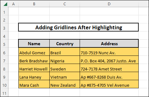
Our sample dataset contains the names, countries, and addresses of five people. We can highlight the data in our sample dataset by following these steps.

• To highlight our data, we select the cell range B6:D10 and go to the Font section under the Home tab.
• Then, we select the Fill Color option and pick a suitable color. We pick the following color shown in the image below.

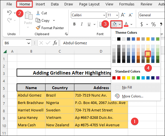
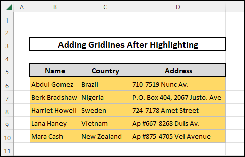
• Thus, our selected cells will be highlighted.

Learn to Add Gridlines After Highlighting Cells in Excel with These 5 Approaches

The cells in our dataset have been highlighted. We will use this modified dataset to add gridlines in Excel. We will thus, look at how we can add gridlines after highlighting using these five approaches.

The Borders section will allow us to select and customize the borders of a cell or multiple cells. We will find the Border option from the Font section under the Home tab to add borders to the highlighted cells in our data. To do so, we follow these steps.

⬇️⬇️ STEPS ⬇️⬇️

• In the beginning, we select the highlighted cells of range B6:D10.
• Next, we go to the Font section under the Home tab.
• We select the Border option and click on All Borders.

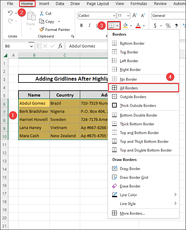
• We will see that the highlighted data have gridlines visible like the following image.

The Border option is also accessible through Format Cells feature. This option allows us to customize the borders and gridlines according to our needs. The option is also accessible by pressing the shortcut key Ctrl+1. The steps for adding gridlines to highlighted cells in this approach are as follows.

⬇️⬇️ STEPS ⬇️⬇️

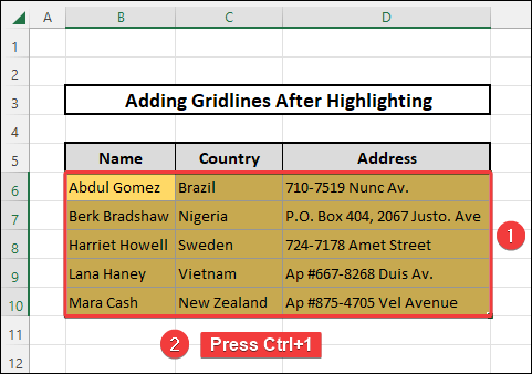
• At first, we select the highlighted cells and press the shortcut key Ctrl+1.

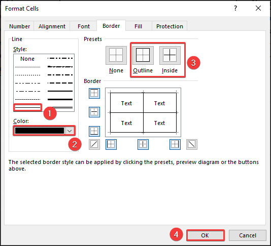
• The Format Cells window will appear. In the Border menu, we select the following Line Style and pick a color.
• After that, we select both the Outline and the Inside options from the Presets category and press OK.

• We observe that our highlighted dataset has gridlines now.

We can create a custom cell style and later select that style for our desired cells to add gridlines in Excel after highlighting. This custom cell style can be useful in ways that if we save it, we can use it later as well. The steps for this approach are as follows.

⬇️⬇️ STEPS ⬇️⬇️

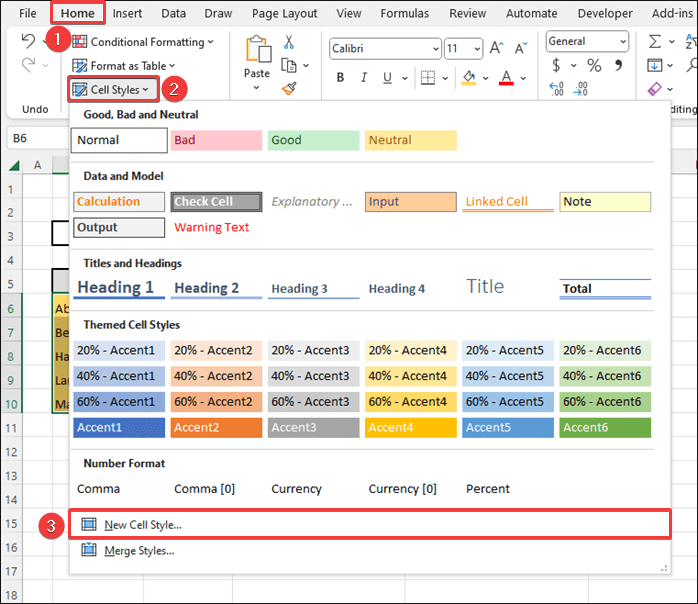
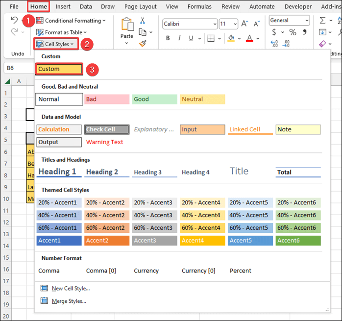
• At first, we go to Home tab and click on Cell Style option under the Styles section.
• The Cell Style drop-down menu will appear. We select the New Cell Style option.

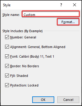
• A Style box will pop up. We name the new style as Custom and click on the Format button.

• A Format Cells box will appear.
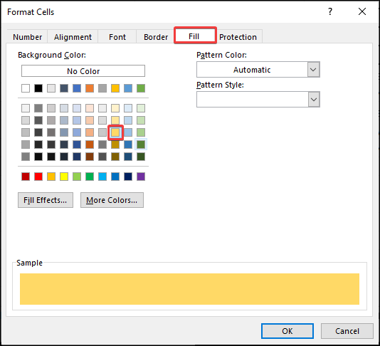
• In the Fill section, we pick the same color as the highlighted color as shown in the following image.

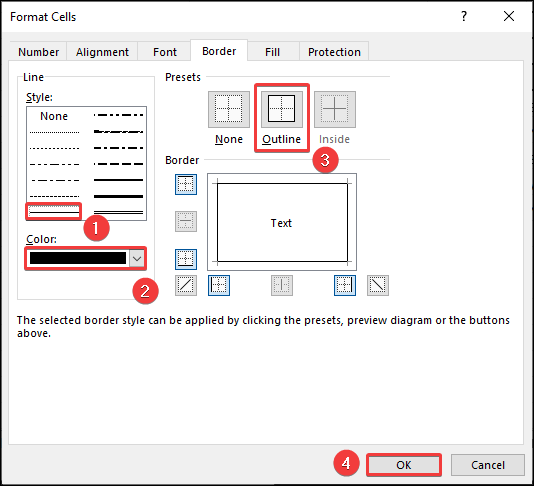
• Then, we move on to the Border section of the Format Cells box.
• We select a line style and color of that line. In the Presets section, we select the Outline option and press OK.

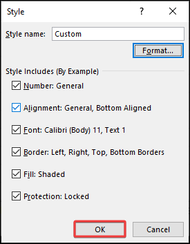
• We press OK button on the Style window.

• First, select the cell range B6:D10.
• From the Cell Style option under the Styles section, we select the Custom cell style.

• The resultant output will have gridlines as shown in the following image.

Using shortcut keys can be an easy way to add gridlines in Excel after highlighting. This shortcut key works in the same way that we can add the All Borders option from the Border drop-down menu under the Home tab.

⬇️⬇️ STEPS ⬇️⬇️

• Firstly, we select the range of cells around which we want to add gridlines.
• In this case, we select the cell range B6:D10.
• After that, we press the shortcut key Alt+H+B+A in sequential order.

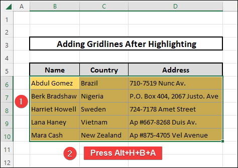
• We will observe that the selected cell range will now have gridlines added across the cell boundaries.

📕 Read More: 2 Approaches to Add More Gridlines in Excel

The Format as Table option lets us select various table styles. It is present in the Styles section under the Home tab. We can use this option to add gridlines to highlighted cells as well. The steps for this approach are as follows.

⬇️⬇️ STEPS ⬇️⬇️

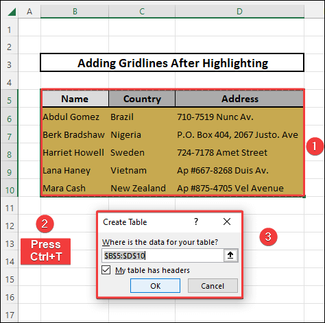
• At first, we select the entire dataset within the cell range B5:D10.
• Then, we press the shortcut key Ctrl+T. A popup box named Create Table will be formed.
• We check on the option My table has headers.

• The dataset will be converted into a table.
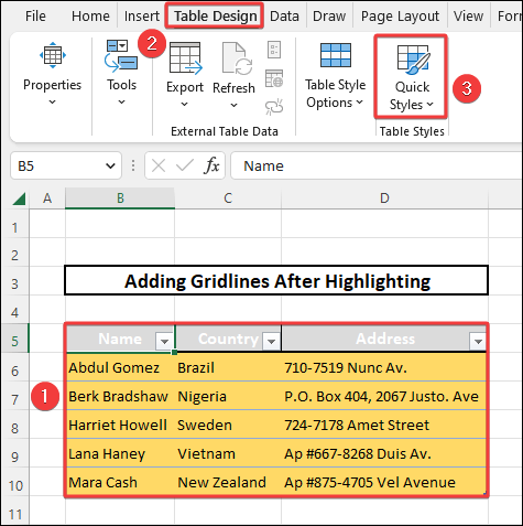
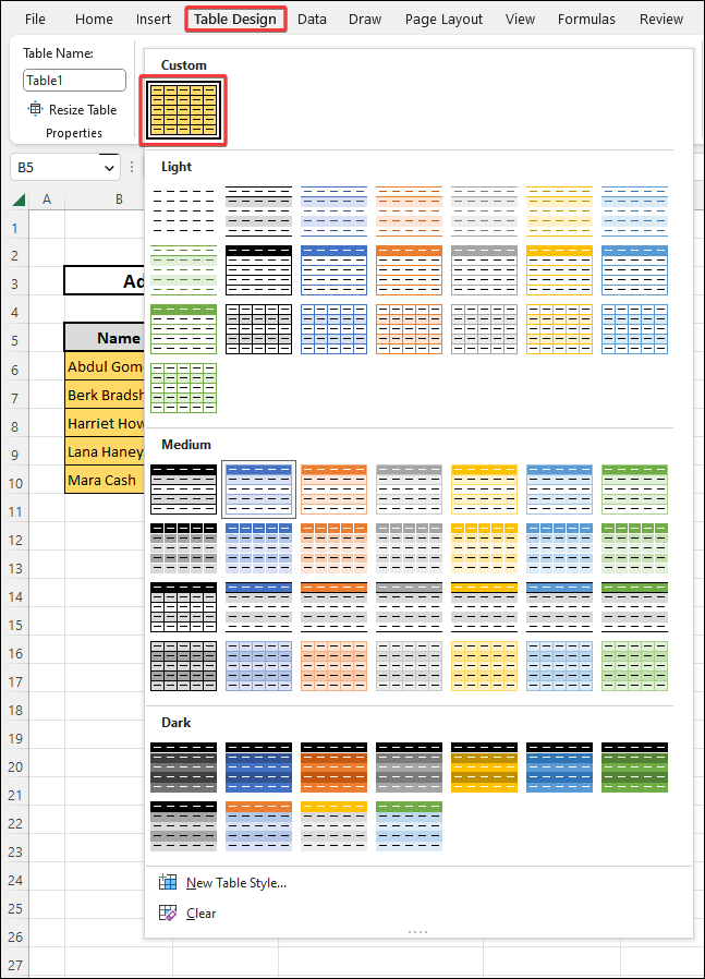
• Now, we hover over to the Table Design tab.
• From the Table Styles drop-down menu, we select Quick Styles option.

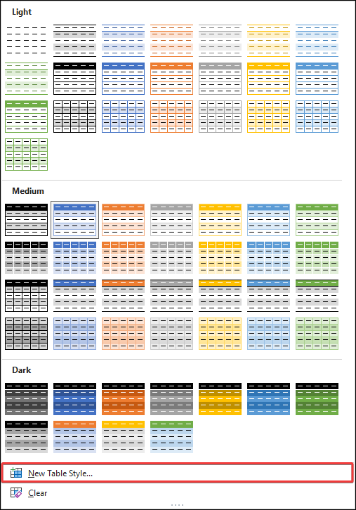
• From the drop-down menu, we select the option New Table Style.

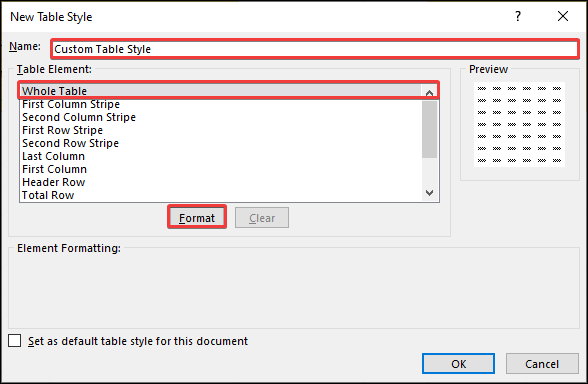
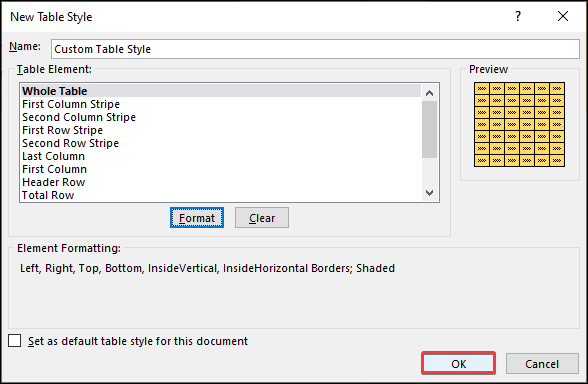
• A New Table Style window will appear. We write the name of the custom style as Custom Table Style.
• Then, we select the Table Element as Whole Table and click on the Format option.

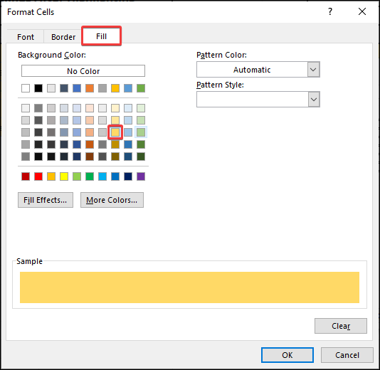
• From the Fill section, we select the color in which the cells were highlighted.

• From the Border section, we select the Line Style as a solid line and Color as black.
• Again, from the Presets category, we select both the Outline and the Inside options and press OK.

• In the New Table Style, we press OK again.

• Now, with the selected data table, we go to the Table Styles option again under the Table Design menu.
• From the drop-down menu, we select the Custom table style.

• Thus, in this way, we can add gridlines in Excel after highlighting using Format as Table option.

📕 Read More: 2 Approaches to Add Primary Minor Vertical Gridlines in Excel

How to Change Color of Gridlines in Excel

The gridline that is shown in general is set to an automatic color. We can change the default color of the gridlines by following these steps.

⬇️⬇️ STEPS ⬇️⬇️

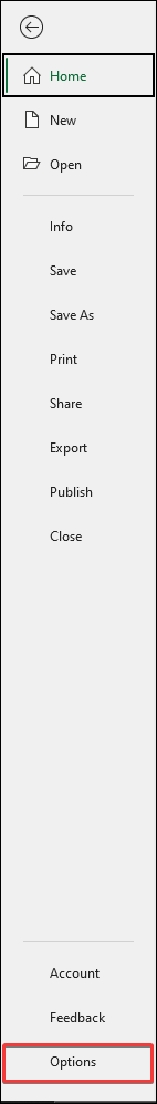
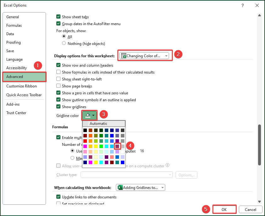
• We go to Options from the File tab of Excel.

• Then, we go to the Advanced section of Excel Options.
• Under the Display options for this worksheet category, we select our present worksheet named Changing Color of Gridlines.
• In the Gridline color section, we click on the drop-down menu and select a suitable color.
• After that, we press OK.

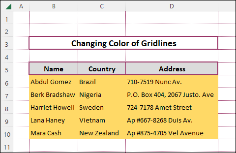
• We will see that the gridlines of that worksheet will change into a different color as shown in the following image.

📄  Important Notes

🖊️  When we use the Format as Table option to add gridlines to highlighted cells, we must convert the dataset into a table first by pressing Ctrl+T.

🖊️  Apart from the All Borders shortcut key, we can use the shortcuts Alt+H+B+O, Alt+H+B+P, Alt+H+B+L, and Alt+H+B+R to add borders only to the bottom, top, left, and right of the selected cells respectively.

🖊️  If the gridlines are not visible, we can check the Gridlines option from the View tab.

📝  Takeaways from This Article

You have taken the following summed-up inputs from the article:

📌  We can add gridlines after highlighting cells in Excel by changing the Border type directly or by using the Format Cells option that can be found by selecting the More Borders option from the Font section of the Home tab.

📌  We can also use shortcut keys to add different types of borders on gridlines.

📌  Using Custom cell styles, we can add gridlines to highlighted cells as well.

📌  Additionally, the Format as Table option can also be useful in adding gridlines after highlighting cells in Excel.

Conclusion

To conclude, I hope that this article has helped you to understand how to add gridlines after highlighting cells in Excel and also how we can change the color of the gridlines in Excel. If you have any queries, reach out to us by leaving a comment below. Follow our website ExcelDen for more informative articles related to Excel.