In this lesson, I’ll demonstrate 11 effective approaches to compare addresses in Excel. Moreover, these techniques will enable you to solve the problem that led you here. However, you will master several crucial Excel features and functions during this article, which will come in extremely handy for any assignment using Excel.
📁 Download Excel File
The sample worksheet that was used during the discussion is available to download for free right here.
Learn to Compare Addresses in Excel with These 11 Useful Techniques
Here, in this article, we will learn how to compare addresses in Excel using different approaches. To be exact, I’ve provided a total of 11 methods down below.
1. Using Built-in Features
We are going to compare Addresses using the built-in feature of Excel here which is Conditional Formatting. In this approach, we format cells as a product of the result.
1.1 Conditional Formatting with Basic Options
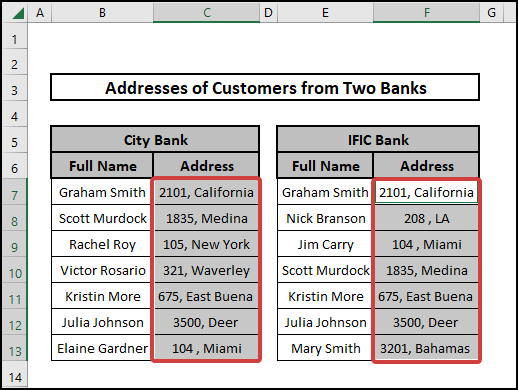
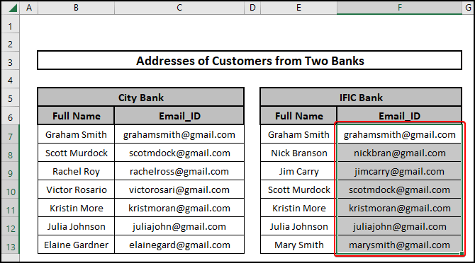
Let’s say we have a dataset that has the list of customers and their addresses for Two Banks. Now we will determine which addresses are common in both lists.
⬇️⬇️ STEPS ⬇️⬇️
- Firstly, select the columns having addresses you want to compare by selecting pressing Ctrl.
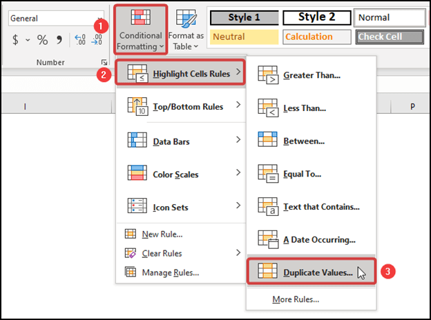
- After that go to Home Tab. On the right side of the ribbon, you’ll find an option named Conditional Formatting. Now choose Highlight Cells Rules and then Duplicate Values like the picture below.
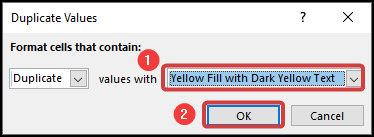
- A new window will pop up. Now select Yellow Fill with Dark Yellow Text in the values with the option and then click OK.
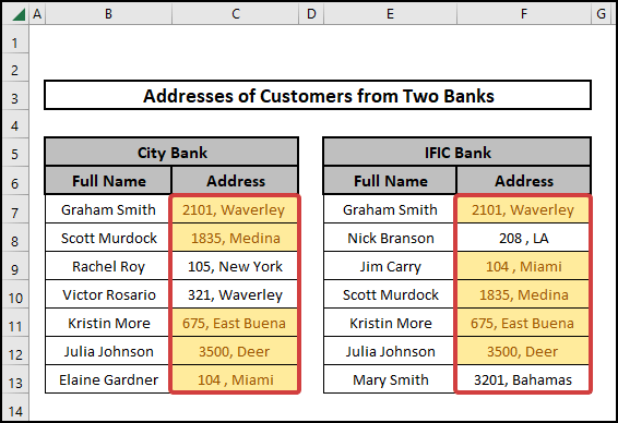
- After that, you will see the following results.
1.2 Conditional Formatting with Formula
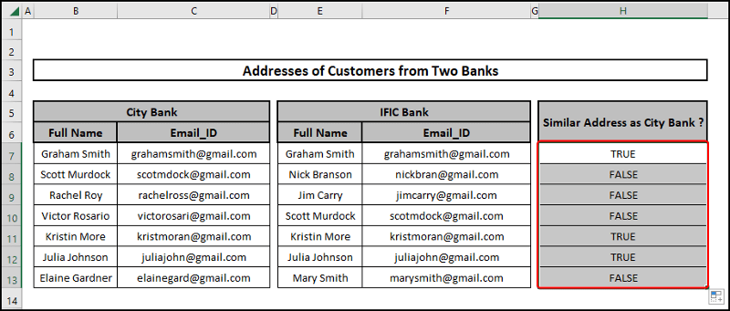
In this section, we will be using the conditional formatting tool with a formula to compare E- mail addresses in Excel.
⬇️⬇️ STEPS ⬇️⬇️
- First, Select the whole column you want to check for similarities.
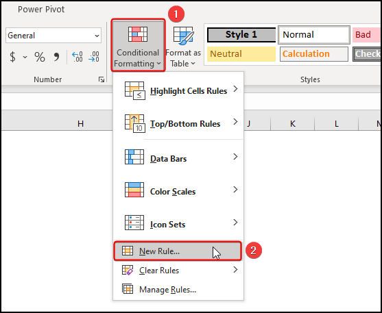
- After that go to Home Tab. On the right side of the ribbon, you’ll find an option named Conditional Formatting. Then select New Rule like the picture below.
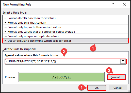
- Now a new window will appear copy the following formula for comparing addresses. Change the Preview Format as per your choice.
=ISNUMBER(MATCH(F7, $C$7:$C$13,0))
🔨 Formula Breakdown
👉 MATCH(F7, $C$7:$C$13,0)
The MATCH function searches for F7 in the range $C$7:$C$13 and returns the position of the searched item which is the ROW number and 0 defines that it identifies the biggest value that is lower or equivalent to the lookup value.
👉 ISNUMBER(MATCH(F7, $C$7:$C$13,0))
The ISNUMBER function tells us if the value is a number or not by TRUE and FALSE.
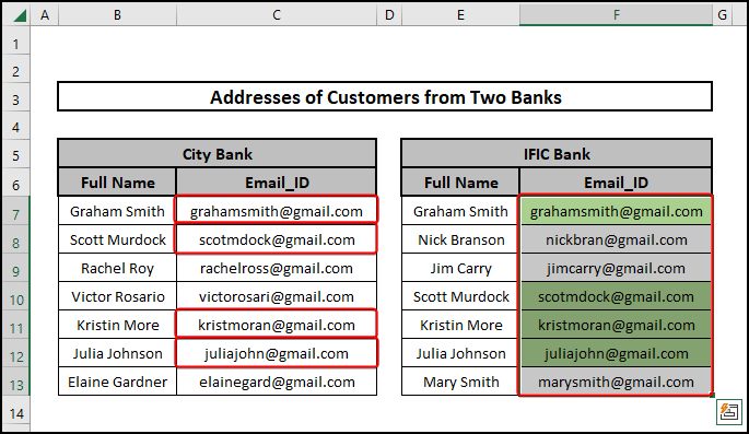
- Once you have done you’ll see the following results.
📕 Read More: 6 Easy Methods to Compare Two Strings in Excel for Similarity
2. Using Excel Formulas
Our goal here is to learn how to compare addresses in Excel. Now in this section, we are going to learn how to use different functions to make effective formulas to compare addresses. We will see the use of some basic functions such as IF, COUNTIF, ISNUMBER, MATCH, XMATCH, ISTEXT, VLOOKUP SUBSTITUTE, LOWER, and LEFT Functions.
2.1 Using the Equal Operator
Here, we will be comparing the addresses of the customers from two different Banks using the Equal Operator. It is a very straightforward process we are just comparing cells that are of the same row for this method.
⬇️⬇️ STEPS ⬇️⬇️
- Firstly, copy the following formula to a cell.
=C7=F7
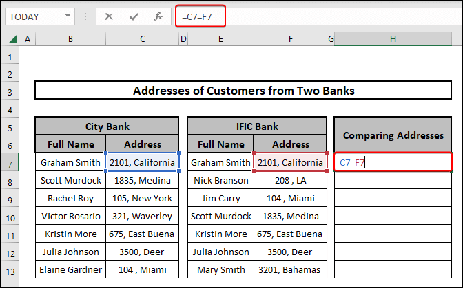
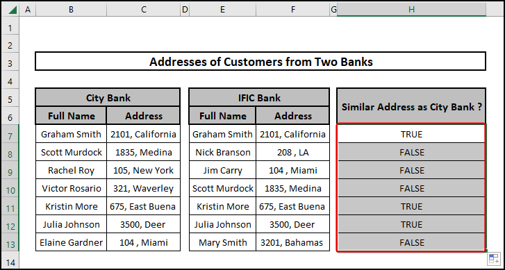
- Press Enter and copy down the formula along the column to get the results as TRUE/FALSE.
2.2 Using IF Function
Now we will be using a formula by the IF Function to find if the customer details for the two Banks’ data are same or not. It’s a straightforward method that just compares two cells in a row.
⬇️⬇️ STEPS ⬇️⬇️
- First, select a cell and copy the following formula I’ve made here for you.
=IF(C7=F7,”Same”,”Different”)
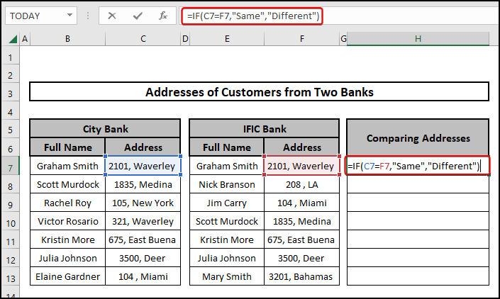
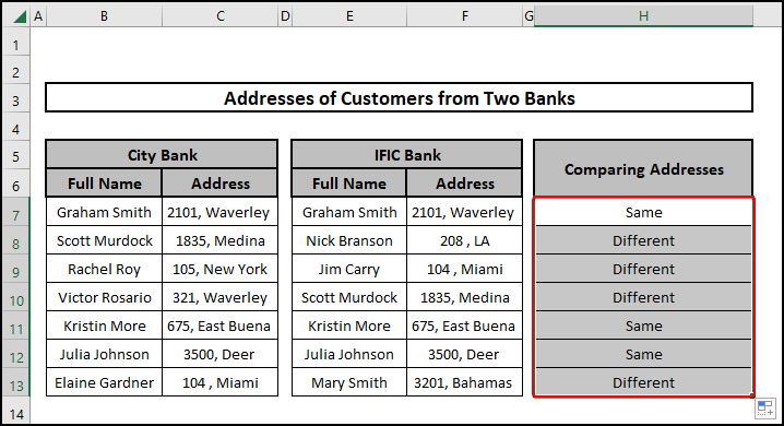
- Press Enter and copy down the formula along the column for all the results.
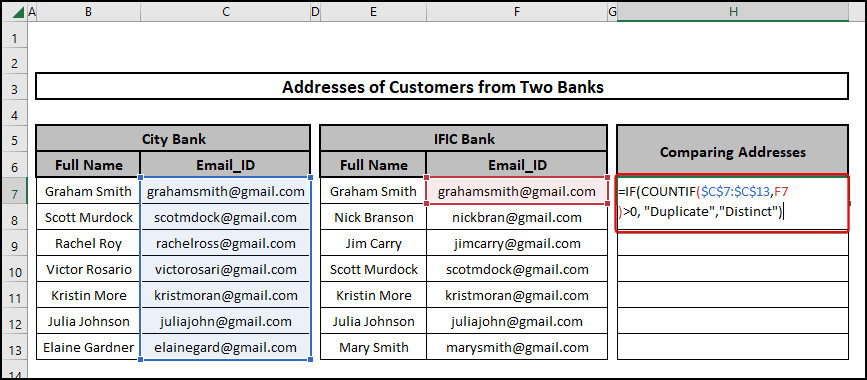
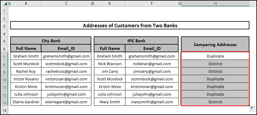
2.3 With COUNTIF Function
Now we are going to use the COUNTIF Function to compare addresses in excel. This function counts the number of cells that meets certain criteria. We are going to use the IF function to show results based on our criteria.
⬇️⬇️ STEPS ⬇️⬇️
- Select and copy the following formula here I’ve prepared for you.
=IF(COUNTIF($C$7:$C$13,F7)>0, “Duplicate”,”Distinct”)
🔨 Formula Breakdown
👉 COUNTIF($C$7:$C$13,F7)
The COUNTIF function counts the number of cells that are similar to F7 in the range $C$7:$C$13.
👉 IF(COUNTIF($C$7:$C$13,F7)>0, “Duplicate”,”Distinct”)
This part says if the number count by the COUNTIF function is bigger than 0 then it will show Duplicate else Distinct.
- Press Enter and copy down the formula along the column for all the results.
📕 Read More: How to Compare Two Cells in Different Sheets with Excel Formula
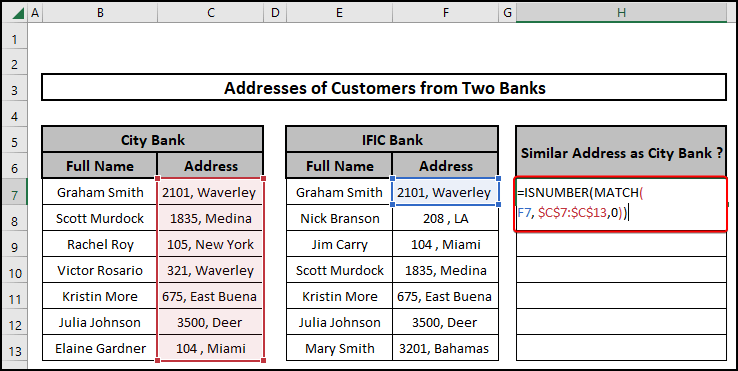
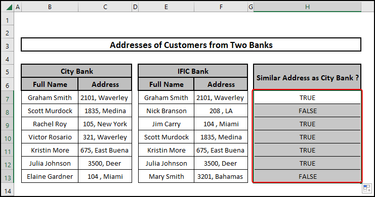
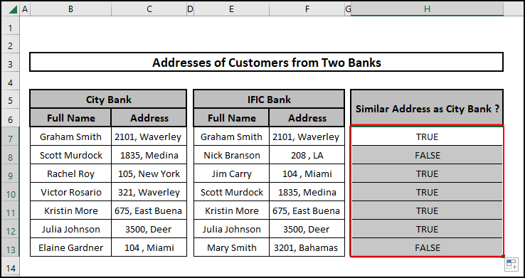
2.4 Merging ISNUMBER and MATCH Functions
This time, we will demonstrate an approach using ISNUMBER and MATCH functions. Here MATCH function searches for a specific value and the ISNUMBER function tells whether it’s a number or not. Thus the answers will be TRUE/ FALSE
⬇️⬇️ STEPS ⬇️⬇️
- Firstly select and copy the formula I’ve given below here.
=ISNUMBER(MATCH(F7, $C$7:$C$13,0))
🔨 Formula Breakdown
👉 MATCH(F7, $C$7:$C$13,0)
The MATCH function searches for F7 in the range $C$7:$C$13. It returns the positions of the searched item. Which are the ROW number and 0 defines that it identifies the biggest value that is lower or equivalent to the lookup value.
👉 ISNUMBER(MATCH(F7, $C$7:$C$13,0))
The ISNUMBER function tells us if the value is a number or not by TRUE and FALSE.
- Press Enter and copy down the formula along the column for all the results.
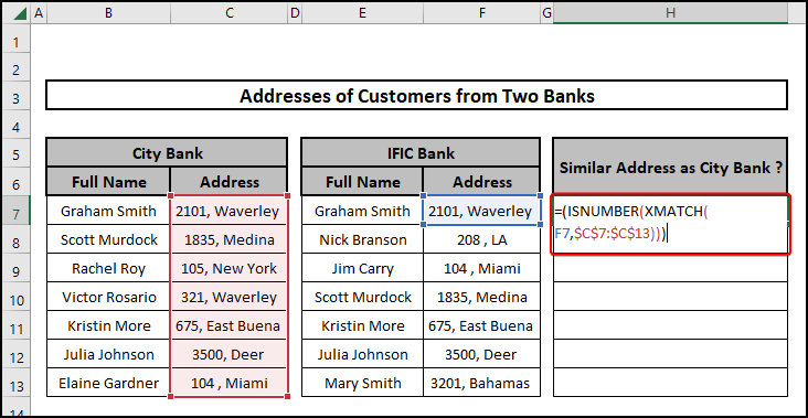
2.5 Combining ISNUMBNER and XMATCH Functions
This method is quite similar to the past method which was using ISNUMBER and MATCH. Here, we will be using XMATCH instead of the MATCH function.
⬇️⬇️ STEPS ⬇️⬇️
- Firstly, select and copy the following formula I’ve provided here.
=(ISNUMBER(XMATCH(F7,$C$7:$C$13)))
🔨 Formula Breakdown
👉 XMATCH(F7,$C$7:$C$13)
The XMATCH function searches for F7 in the range $C$7:$C$13. It returns the relative position of the searched item. Which is the relative ROW number.
👉 (ISNUMBER(XMATCH(F7,$C$7:$C$13)))
The ISNUMBER function tells us if the value is a number or not by TRUE and FALSE.
- Press Enter and copy down the formula along the column for all the results.

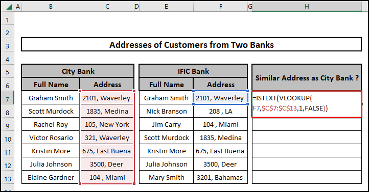
2.6 Integrating ISTEXT and VLOOKUP Functions
Here we are going to use ISTEXT and VLOOKUP functions to compare the addresses of the two Banks’ customers. Here VLOOKUP searches for the value we command it and ISTEXT checks whether the value is TEXT or not.
⬇️⬇️ STEPS ⬇️⬇️
- First, select and copy the following formula I’ve provided here.
=ISTEXT(VLOOKUP(F7,$C$7:$C$13,1,FALSE))
🔨 Formula Breakdown
👉 VLOOKUP(F7,$C$7:$C$13,1,FALSE)
The VLOOKUP function looks up for the EXACT value (as it says FALSE) F7 in the 1st column from the range $C$7:$C$13 the highest value in the array $C$6:$C$14.
👉 ISTEXT(VLOOKUP(F7,$C$7:$C$13,1,FALSE))
The ISTEXT function tells us if the value is a TEXT or not by TRUE and FALSE.
- Press Enter and copy down the formula along the column for all the results.
2.7 Using LEFT Function
Here we are going to use the LEFT function to compare between addresses. This function returns the leftmost value of a cell. If we use a comma then it can return values that have specific numbered characters. For instance, the formula used here is checking if a 5-char word of cell C7 and a 5-char word of cell F7 are equal or not.
⬇️⬇️ STEPS ⬇️⬇️
- First, select and copy the following formula I’ve provided here.
=LEFT(C7,5)=LEFT(F7,5)
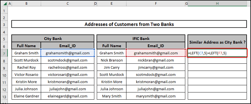
- Press Enter and copy down the formula along the column for all the results.
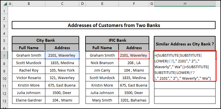
2.8 Combining SUBSTITUTE and LOWER Functions
A different approach to compare addresses using SUBSTITUTE and LOWER functions.
⬇️⬇️ STEPS ⬇️⬇️
- Firstly, select and copy the following formula I’ve provided here.
=(SUBSTITUTE(SUBSTITUTE(LOWER(C7),”2101″,”2″),”Waverly”,”Wa”))=SUBSTITUTE(SUBSTITUTE(LOWER(F7),” 2101″,” 2″),” Waverly”,” Wa”)
🔨 Formula Breakdown
👉 LOWER(C7)
The LOWER function converts all uppercase letters to lowercase letters of cell C7.
👉 SUBSTITUTE(LOWER(C7),”2101″,”2″)
LOWER C7 is a lowercase-based value. This part says that 2101 is now substituted by 2 of the cell LOWER C7
👉 SUBSTITUTE(SUBSTITUTE(LOWER(C7),”2101″,”2″),”Waverly”,”Wa”)
This says that the Substitute in C7 will be again substituted. Old text is Waverly new text is Wa.
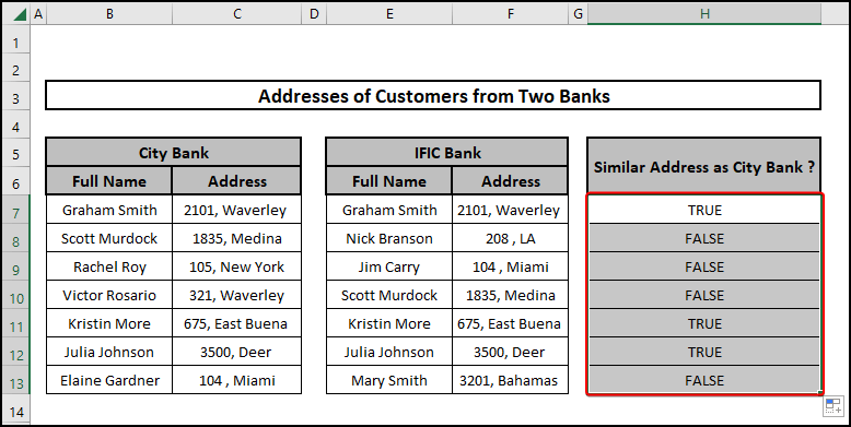
👉 (SUBSTITUTE(SUBSTITUTE(LOWER(C7),”2101″,”2″),”Waverly”,”Wa”))=SUBSTITUTE(SUBSTITUTE(LOWER(F7),” 2101″,” 2″),” Waverly”,” Wa”)
This formula defines if both the logics are equal on C7 and F7. If they are equal the formula returns TRUE and if not it returns FALSE.
- Press Enter and copy down the formula along the column for all the results.
3. Using VBA
We can always use VBA codes to solve any kind of problem. VBA is an advanced professional feature of Microsoft Excel. As we have learned all other possible methods except this one.
⬇️⬇️ STEPS ⬇️⬇️
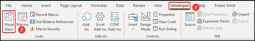
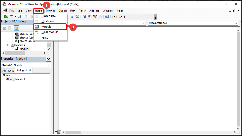
- Firstly, you have to enable the Developer Tab in your Excel to use VBA. Then Go to the Visual Basic option from the Developer Tab of the ribbon.
- After that, a window will pop up, go to Module from the Insert option like the picture below.
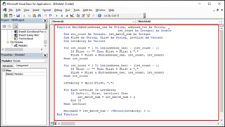
- Copy the following VBA Code in the Module.
Function MatchAdd(address_one As String, address_two As String, _
    let_count As Integer) As Double
    Dim int_count As Integer, let_match_num As Integer
    Dim FList As String, SList As String, LettList As Variant
    Dim LettArray As Variant
    For int_count = 1 To Len(address_one) - (let_count - 1)
        If FList <> "" Then FList = FList & ","
        FList = FList & Mid(address_one, int_count, let_count)
    Next int_count
    For int_count = 1 To Len(address_two) - (let_count - 1)
        If SList <> "" Then SList = SList & ","
        SList = SList & Mid(address_two, int_count, let_count)
    Next int_count
    LettArray = Split(FList, ",")
    For Each LettList In LettArray
        If InStr(1, SList, LettList) Then
            let_match_num = let_match_num + 1
        End If
    Next LettList
    MatchAdd = let_match_num / (UBound(LettArray) + 1)
End Function
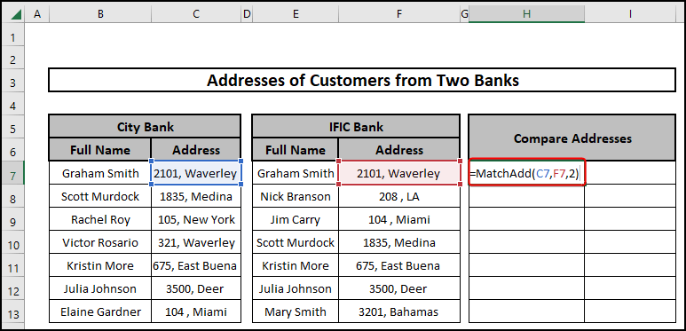
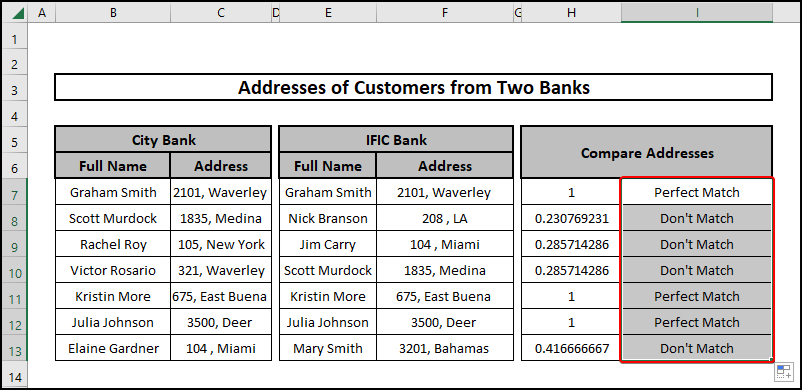
- Now after saving the code we have successfully created a custom function that we can use to compare addresses as it finds the percentage of strings and characters matched on a scale of 1.
=MatchAdd(C7,F7,2)
- After copying the custom function along the column. now we will add some conditions to it according to its matching ratio to get the comparison.
=IF(MatchAdd(C7,F7,2)=1,”Perfect Match”,”Don’t Match”)
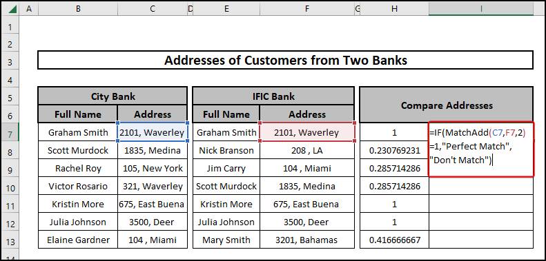
- Press Enter and copy down the formula along the column for all the results.
📄 Important Notes
🖊️ Be careful while using the code as there are a lot of terms and if you lose concentration the code may be incorrect.
🖊️ Use shortcuts to reduce time, and use F4 for absolute value.
🖊️ While writing formulas carefully see the suggestions and don’t forget the commas and parentheses.
🖊️ Be careful while defining criteria to be accurate as the dataset.
🖊️ If you download a macro-enabled Excel file don’t forget to unblock the file from the properties menu.
📝 Takeaways from This Article
📌 Use of IF, COUNTIF, ISNUMBER, MATCH, XMATCH, ISTEXT, VLOOKUP SUBSTITUTE, LOWER and LEFT functions.
📌 How to Compare both E-mail Addresses and Living Addresses
📌 Creating formulas using multiple functions.
📌 Using VBA codes to customize functions.
📌 How to define a new function.
📌 Conditional formatting and its usage to sort things out.
📌 Conditional formatting defines any formula.
Conclusion
Firstly, I hope you were able to use the techniques I demonstrated in this how-to compare addresses in the Excel lesson. As you can see, there are a lot of options on how to do this. However, decide deliberately on the approach that best addresses your circumstance. Most importantly I advise repeating the steps if you become confused in any of the steps if you get stuck. Practice on your own after looking at the Excel file in the practice workbook, I’ve provided above because practice makes a man perfect. Above all, I earnestly hope you can use it. Please share your experience with us in the comments about how your experience was throughout the article and what we need to improve or add to make things better for you folks. However, if you have any problem regarding Excel spit it in the comment box. The Excelden crew is always available to answer your questions. In conclusion, keep educating yourself by reading. For more Excel-related articles please visit our website Excelden.com.
Related Article


