12 Quick Tricks to Create a Formula in Excel for Multiple Cells

Are you a student? Do you work for any financial Institution? Or, conduct scientific research? Here one thing is common among all these professionals that are everyone has to deal with data. On the other hand, MS Excel is the most widely used software to work with data. During dealing with data one must create a formula for multiple cells in Excel. To create a formula in Excel for multiple cells, there are several approaches everyone should know.

📁 Download Excel File

To practice please download the excel file from here:

Learn to Create a Formula in Excel for Multiple Cells in 12 ways

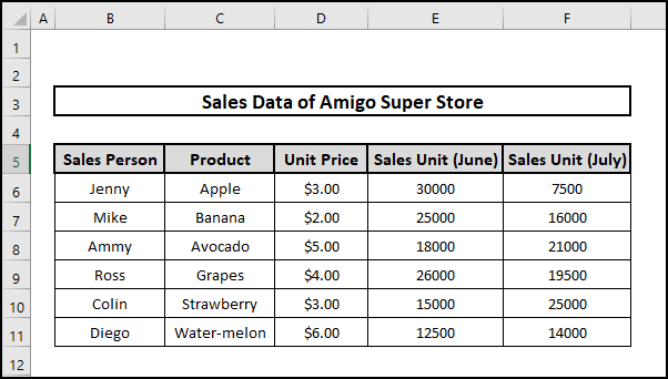
We are going to crack 12 approaches to create a formula in Excel for Multiple Cells. We are considering a dataset named Sales Data of Amigo Super Store. The Dataset table contains Sales person, Product, Unit Price, Sales Unit (June), and Sales Unit (July). Dataset also has 6 columns and 11 rows. We are going to discuss several methods briefly including VBA. So let’s get started.

Just clicking with your mouse and auto-filling with the Fill Handle you can generate simple formula. Let’s follow the steps,

 ⬇️⬇️ STEPS ⬇️⬇️

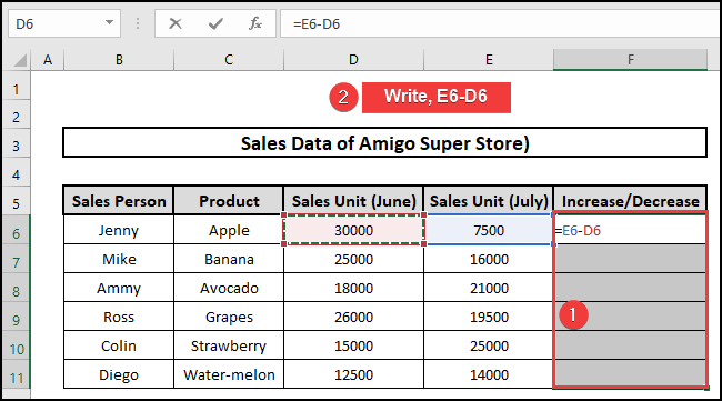
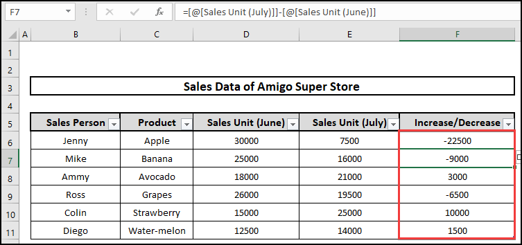
• First, select a blank cell i.e. F6.
• Then insert an Equal Sign (=).
• Next, Select E6, type Minus (-), and select D6.

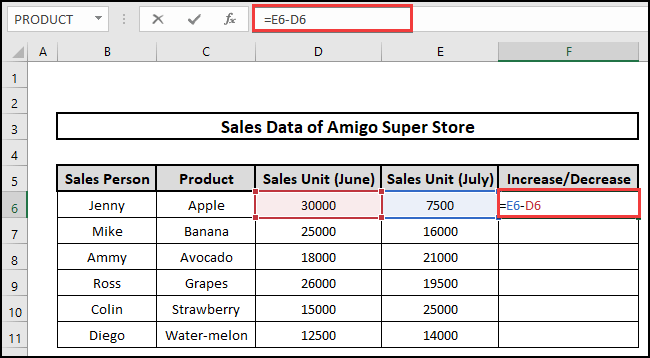
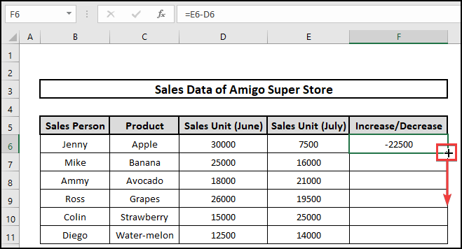
• You will get -22500 in F6 That indicates a decrease with respect to the Sales Unit of the previous month June.
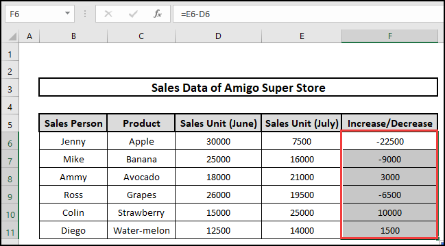
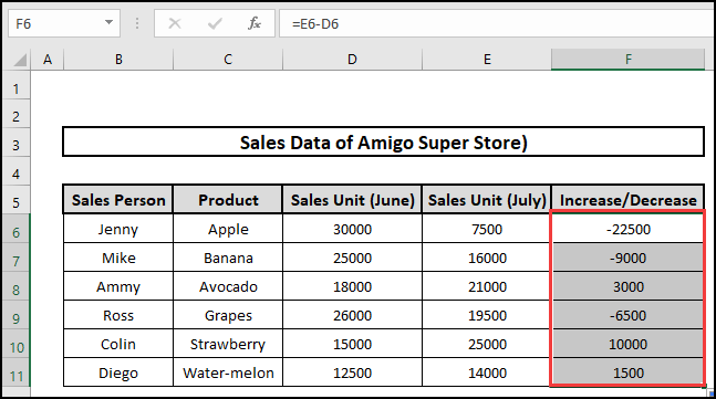
• After that, Using Fill Handle, you get the value for each cell.

• Thus, you get the full results.

Selecting the whole column of the table and inserting the simple formula, one can get the total output very easily. Let us follow the below steps.

 ⬇️⬇️ STEPS ⬇️⬇️

• Initially, select a blank cell range F6:F11.
• Then type the following formula to get into the output range.

• Finally, in the F6:F11 range, we get the results sequentially.

By creating a table, one can create a formula without any hustle. Please follow the below procedures.

 ⬇️⬇️ STEPS ⬇️⬇️

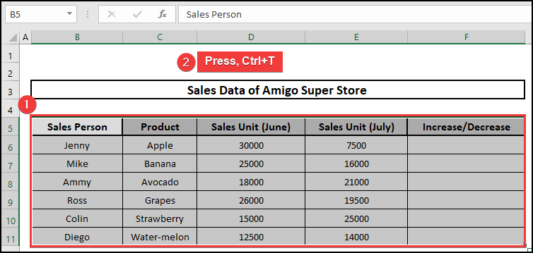
• Primarily select the entire dataset.
• Secondly, Press Ctrl+T to convert the dataset into a table.

• Thirdly, in the F6 cell, insert an Equal Sign (=) first.
• Then Select E6 and type Minus (-), and then select D6.

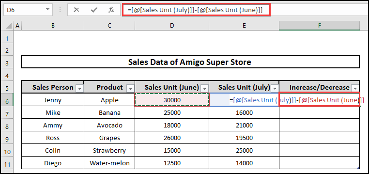
• Finally, the result appears together sequentially.

Selecting the range of the array you can create a formula within a second. Please follow the steps.

 ⬇️⬇️ STEPS ⬇️⬇️

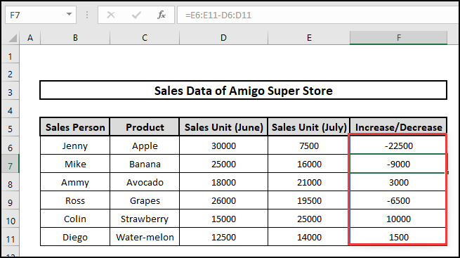
• Firstly, select a blank cell i.e. F6.
• Secondly, insert an Equal Sign (=), select the range E6:E11, type Minus(-), and select the range D6:D11.

• Thirdly, Press Enter.

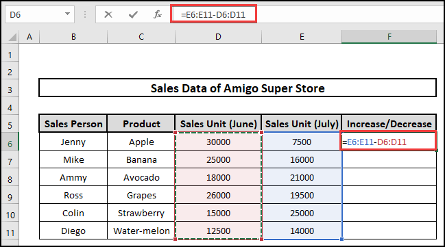
• Finally, You get the full result automatically.

We can use VBA code to create formulas in multiple cells. With the help of the Developer option, you can generate a program of your own. Please follow the steps.

⬇️⬇️ STEPS ⬇️⬇️

• First, Check if your Developer option is available or not.
• Then to enable the Developer option, right-click on the mouse at the top Ribbon and select Customize the Ribbon.

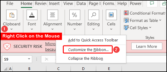
• Click on Developer and click on OK.

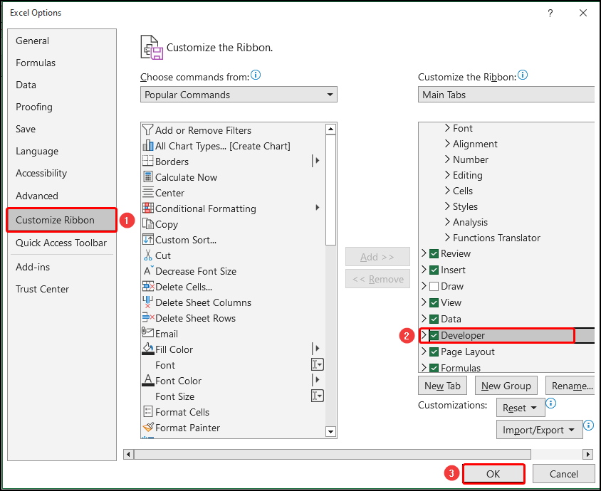
• Now Developer mode is on.
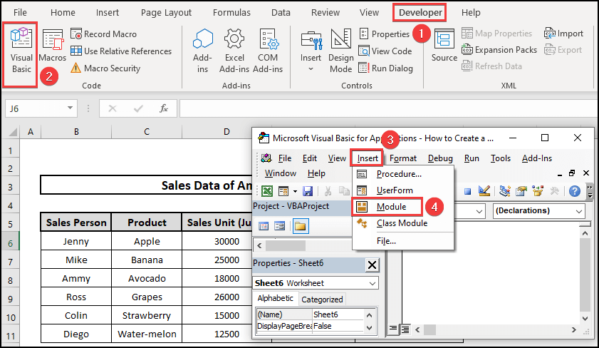
• Click on the Visual Basic option.
• To insert the VBA code, click on Module from the Insert option.

• Insert the following VBA code and click on Run to execute the code.

Code

Sub v_1()
Range("F6").Select
Application.CutCopyMode = False
ActiveCell.Formula2R1C1 = "=RC[-1]:R[5]C[-1]-RC[-2]:R[5]C[-2]"
Range("F7").Select
End Sub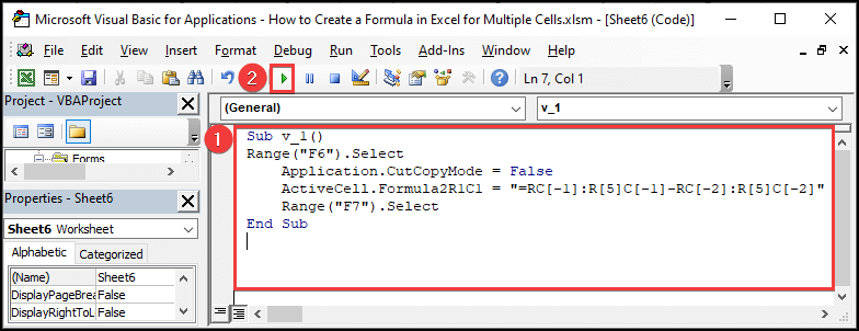

• Finally, we get our desired output at the cell range F6:F11.

Inserting a formula in a particular cell and copying it to other cells with changing cell references can be another way to generate a formula in the entire dataset. Please follow the steps.

⬇️⬇️ STEPS ⬇️⬇️

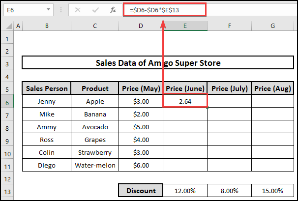
• First, copy the cell’s formula i.e. E6 with the following value.

• Then, auto-fill to the F6 and G6.
• After that copy E6:G6 and Paste it to E7:G7.
• You will get the result with the change of cell references.

• Finally, by auto-filling the table, you will get the final output.

Duplicate cells from the existing formula you can also create a formula for new cells. Please follow the steps.

⬇️⬇️ STEPS ⬇️⬇️

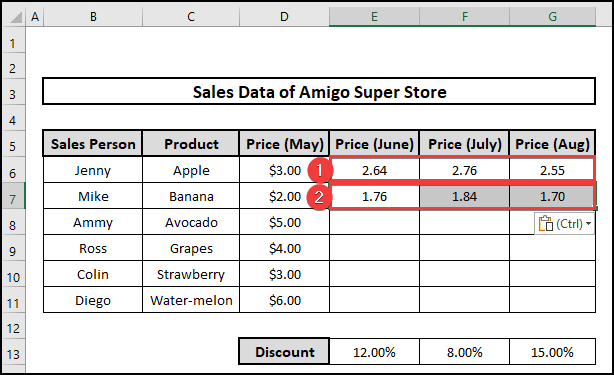
• Primarily, inspect the cell’s formula i.e. E6 with the following value.

• Then selecting each cell in column E, press Ctrl+D to duplicate the formula.

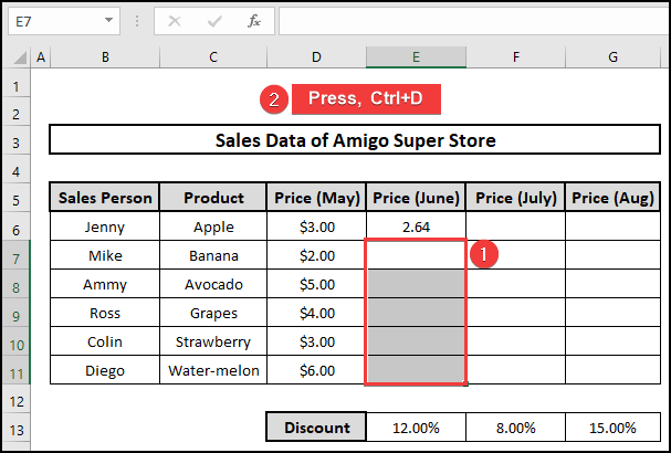
• Therefore, the final result is displayed sequentially cell by cell.

Without copy-paste, we can repeat the previous formula pattern accordingly. Please follow the below procedure.

⬇️⬇️ STEPS ⬇️⬇️

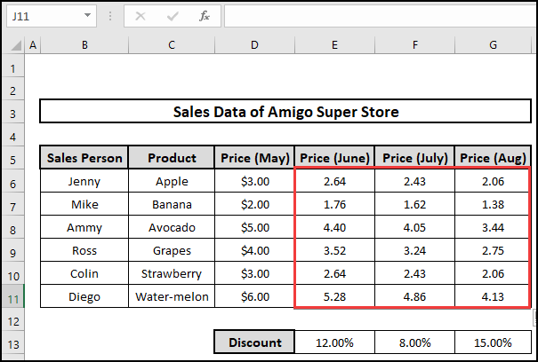
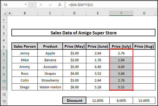
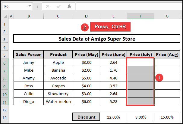
• Primarily, inspect the range’s formula i.e. E6:E11 with the following value.
• Then select the cells to get the output.
• After that, press Ctrl+R to get the repeated pattern of the formula.

• Lastly, we get the final result containing the price of July for each product following the same formula pattern of range E6:E11.

Suppose there are non-adjacent multiple cells. If you calculate it by defining the range, you will get an Error for blank cells. Please follow the procedure to insert the formula to non-adjacent multiple cells in Excel.

⬇️⬇️ STEPS ⬇️⬇️

• Primarily, inspect the cell’s formula i.e. E6 with the following value.
• Secondly, Copy cell E6.
• Thirdly, Hold Ctrl and select the blank cell by clicking.
• Fourthly, Press Ctrl+V to paste the formula of cell E6.

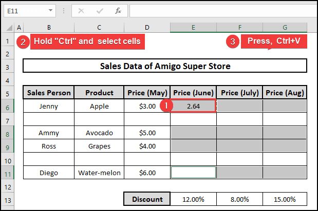
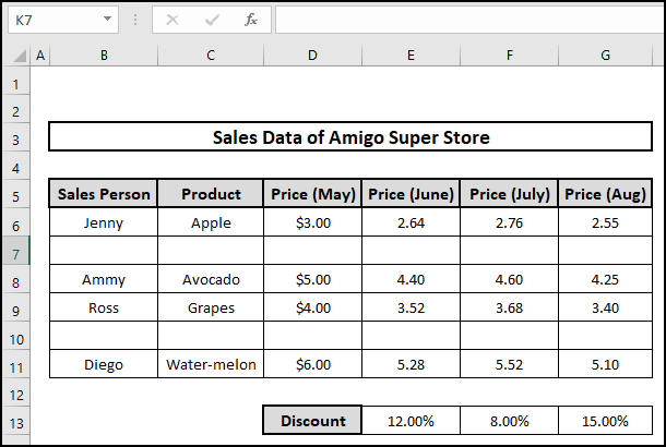
• Finally, we get the value accordingly for every cell.

Suppose you don’t want to type a comma(,) after each cell reference. Using Ctrl+Left-Click(Mouse) can be a way to your calculation. Please follow the steps:

⬇️⬇️ STEPS ⬇️⬇️

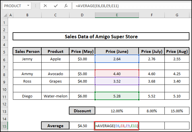
• First, To calculate average of E6, E8, E9 and E11; First write =AVERAGE(
• Then holding Ctrl, select E6, E8, E9, and E11.
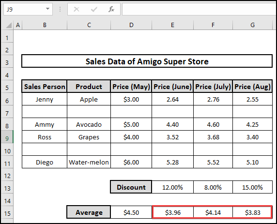
• Now, Press Enter and get the result.

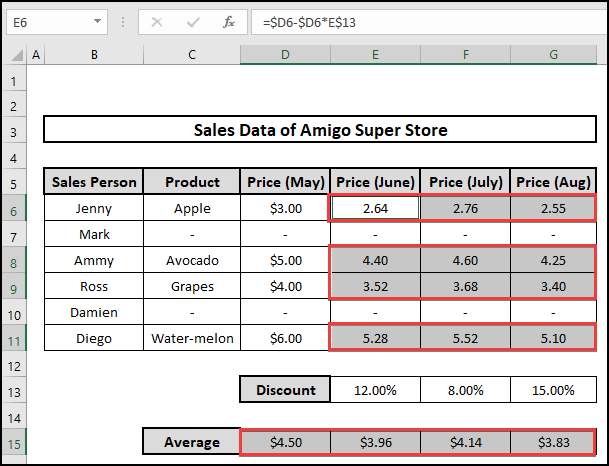
• Auto filling, we obtain the average price for the months of June, July, and Aug.

Suppose you need to find out the cells where formulas are used. To get the cells please follow the steps below,

⬇️⬇️ STEPS ⬇️⬇️

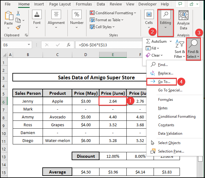
• First, select a cell i.e. E6.
• Next, Select Find and Replace from the Editing menu.
• Then, Click on Go to option.

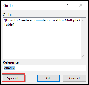
• therefore, a box named Go To appears.
• Now, click on Special.

• A box named Go To Special will appear.
• Select Formulas and click on OK button.

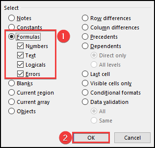
• Therefore cells containing the formula get highlighted.

Sometimes we need to write down complex formulas and we need to evaluate them as well to implement them as a formula. Here follow the necessary procedure.

⬇️⬇️ STEPS ⬇️⬇️

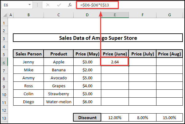
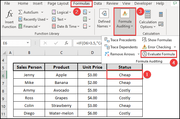
• First, select a cell i.e. E6.
• In E6, the following formula containing the IF function is presented.

• Next, Click on Formula Auditing from Formula Menu at the Top Ribbon.
• Then, click on Evaluate Formula option.

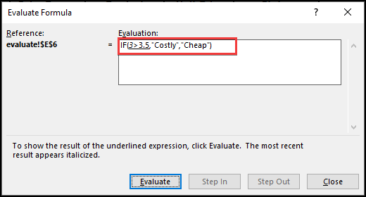
• Now a box appears named Evaluated Formula.
• In the meantime, formula =IF(D6>3.5,”Costly”,”Cheap”) is showing on the box.

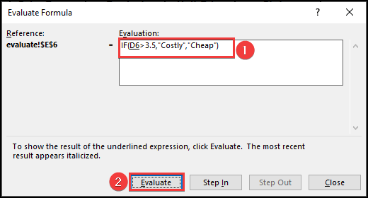
• Click on Evaluate.
• Now it shows the logical expression, =IF(3>3.5,”Costly”,”Cheap”) and writes Cheap as it is 3<3.5.

Following these ways, we can navigate and evaluate any complex formula similarly.

📄 Important Notes

🖊️  Evaluate Formula option is only available on the newer version of MS Excel 365.

🖊️  During working with VBA code, Check first whether your Developer tool is available or not.

📝 Takeaway from This Article

📌  Now you will be able to insert formulas under any circumstances and deal with data.

📌  Evaluate Formula feature can be your best learning during working with complex formulas.

Conclusion

In this article, we demonstrated 12 easy approaches to create formula in Excel for multiple cells. I hope you enjoyed your learning. For better understanding and new learning don’t forget to visit www.ExcelDen.com. Also, leave your thoughts in the comment section.