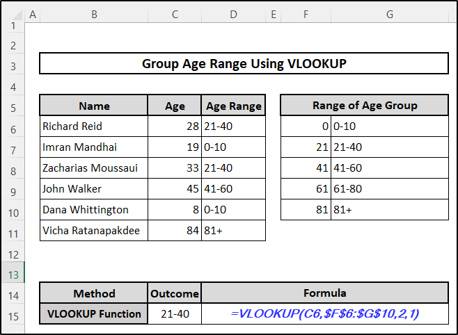
Sometimes you have to deal with a dataset where you have to group the age range. It can be very intimidating if you attempt to do it manually. We suggest you that if you want to group age range in Excel use the function VLOOKUP in this case. In this article, we are going to discuss step-by-step how to group age range in Excel using the VLOOKUP function. Here is the overview of the formula and the output.
📁 Download Excel File
Here is the file that we have used to build this tutorial and you can also use this to learn.
Learn to Group Age Range in Excel Using VLOOKUP Function with These 3 Steps
Suppose, you are given a dataset of people including their Names and Ages. You want to categorize them into ranges or groups. We have mentioned earlier that you can simply use the built-in function of Excel named the VLOOKUP function. In this article, you can find three steps below. Follow those to have an idea of this method.
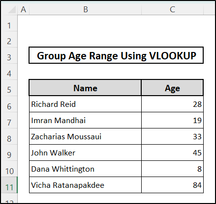
Here is the dataset that we have used in our article.
Step 1: Arranging Data in Excel Sheet
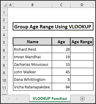
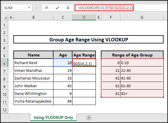
- To range the ages first you have to insert that data and arrange it. Here we have used a dataset of victims of terrorist attacks. The dataset displays their names and ages. Suppose, we want to arrange these data within a range. In this case, we have inserted one column named Age Range where we want to show in which range they belong. So, our dataset is ready.
- Just beside this dataset, we have inserted one table listing the age ranges.
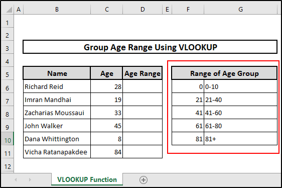
You must insert this table of age ranges in order to insert the function.
Step 2: Apply VLOOKUP Function
- Now as you have inserted the data range and your dataset is ready to write the function. Here we will insert the function under the column of Age Range. You can enter this function in any cell, where you want to see the results.
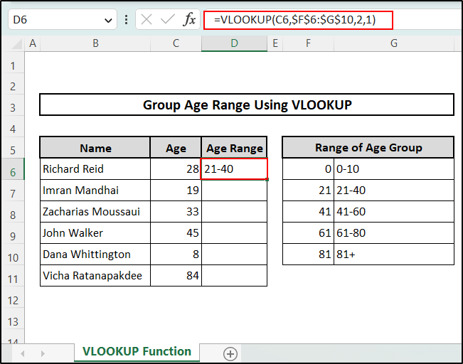
- We have inserted the following formula in cell D6.
=VLOOKUP(C6,$F$6:$G$10,2,1)
🔨 Formula Breakdown
VLOOKUP(C6,$F$6:$G$10,2,1)
👉 Firstly, the syntax of VLOOKUP(lookup_value, table_array, col_index_num, [range_lookup]).
👉 So, according to the syntax of this function lookup_value here is cell C6. This is the value to lookup for.
👉 Next, table_array indicates all the cells of the table. $F$6:$G$10 represents the table where we have stored the data of the age range.
👉 Then, 2 is the col_index_num, which means we are looking at the values of column 2 of the table to find the match with cell C6.
👉 Finally, 1 represents range_lookup. Here, 1 represents TRUE, which means we want this return value to be an approximate match.
- After inserting the function, press Enter from your keyboard.
Step 3: Use Fill Handle Icon to Fill Up the Rest of Cells
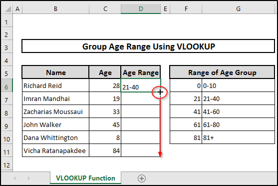
- After entering the formula you have filled only one cell. To perform the same task in the rest of the cells in that column, you have to use the Fill Handle (+) icon.
- Drag this Fill Handle icon downward until all the cells are filled. Here we have dragged this icon up to cell D11.
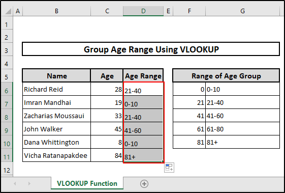
- Finally, you will be able to see the range of the ages where the ages belong.
Group Age Range in Excel Without Using VLOOKUP Function
You can group age ranges in Excel even without using the VLOOKUP function of Excel. In this article, we will discuss three more methods to group age ranges in Excel without inserting any VLOOKUP function.
1. Group Age Range in Excel Using Pivot Table
The Pivot Table is another way to group the age range in Excel. Here, we have used the previous dataset. We want to count the number of people present in a group age range. We have used the Pivot Table to count the number of people in each group age range. Follow the steps below to learn more.
⬇️⬇️ STEPS ⬇️⬇️
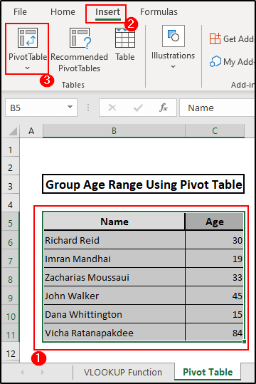
- First of all, select the cells that you are going to use in your Pivot Table. Here, we have selected the cell range B5:C11, as these cells include the data of Age and Name.
- Then, go to the Menu Bar and from there select the option Insert.
- Next, from the Tables group select the Pivot Table.
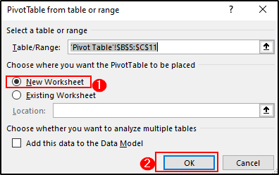
- As a result, a window will pop up named PivotTable from the table or range.
- From there you choose the option where you want to see the pivot table, we have chosen the New Worksheet option for the pivot table to be placed in the new worksheet.
- Then, press OK.
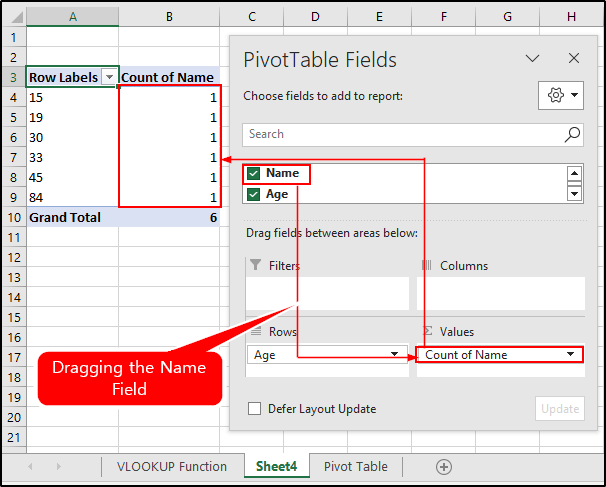
- After that, the Pivot Table Fields will open automatically in the new worksheet.
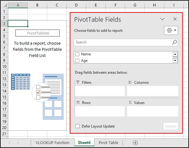
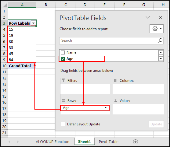
- Now, add the Age under the label Rows, by dragging.
- Again, add the Names under the label Values by dragging.
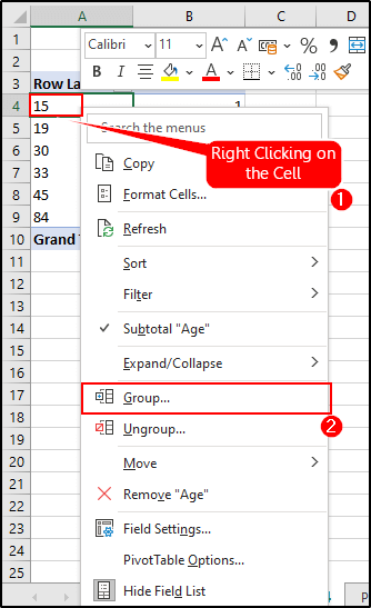
- Then, right-click on the first age data in your Pivot Table and from there select the option, Group.
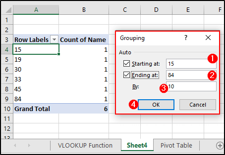
- Due to this a command box named Grouping appears.
- From there you have to select the range of ages. For example, we have inserted 15 in the Starting at and age 84 in the Ending at, which are the lowest and highest values of the dataset.
- Then, the spacing of this data, which is named By is 10. That means our age group range will be counted from the age of 15 with an interval of 10. Also, You can adjust this according to your need.
- Finally, after entering this data you will see that the Pivot Table has counted the number of age data for each range.
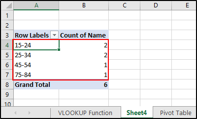
In our dataset, we showed it on the right side of the age range under the title Count of Name.
2. Combining INDEX and MATCH Functions to Group Age Range in Excel
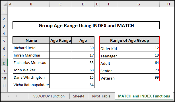
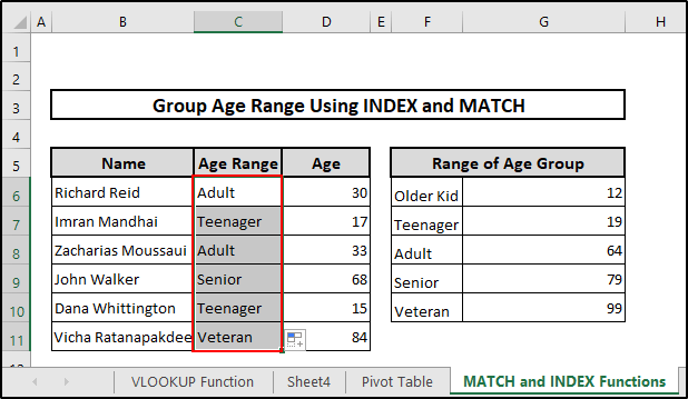
Instead of using the VLOOKUP function, you can use the INDEX and MATCH functions to group age ranges in Excel. Here we have worked with a dataset where we want to determine within which category the ages belong. Follow the steps below to know more.
⬇️⬇️ STEPS ⬇️⬇️
- First, you have to specify the category. For example, here we have inserted a table mentioning which age belongs to which category.
- Then, select the cell where you want to insert the category for your dataset.
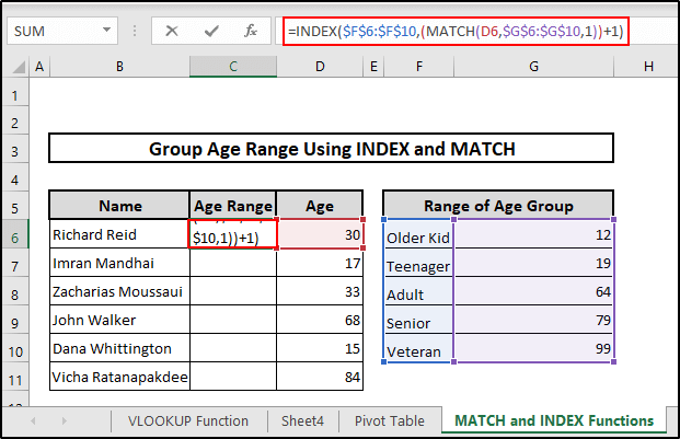
- After that, insert the formula given below.
=INDEX($F$6:$F$10,(MATCH(D6,$G$6:$G$10,1))+1)
🔨 Formula Breakdown
INDEX($F$6:$F$10,(MATCH(D6,$G$6:$G$10,1))+1)
👉 Firstly, from the MATCH(D6,$G$6:$G$10,1) part of the function compared to the syntax of MATCH function is MATCH(lookup_value, lookup_array, [match_type]), where we have taken the cell where the data to be ranged is stored, which is the cell D6.
👉 Here, cell D6 means, it is in the 6th row of the D column.
👉 Then, the range of cells where the value is stored will be searched in the table array $G$6:$G$10.
👉 Finally, the MATCH function will compare these two values and the last match_type part is optional. The default value is 1, which indicates that the MATCH function will find the greatest value and that less than or equal to the lookup_value which is stored in cell D6. So, here is the age stored in D6 which is 30 matches with cell G8 as it is less than 64.
👉 So, here the (MATCH(D6,$G$6:$G$10,1)+1 ) becomes 8, the row_num for the INDEX function.
👉 According to the syntax of the INDEX function, $F$6:$F$10 is the array where the data with which to be compared is stored.
👉 So, the INDEX function will lookup for the 8th row to match with the array and will return its corresponding cell value which is Adult.
- Then, press the Enter button to get the result.
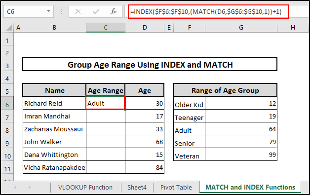
- Now, you can see in which category of age range this specific age belongs. As you can see in this case the age 30 belongs to the Adult age range.
- Finally, use the Fill Handle icon, and drag this icon until the last cell of your dataset to perform the same in all the remaining cells.
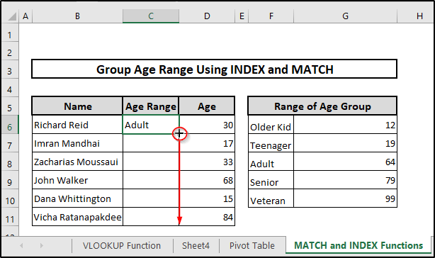
- Now, you can observe that you have filled all other cells.
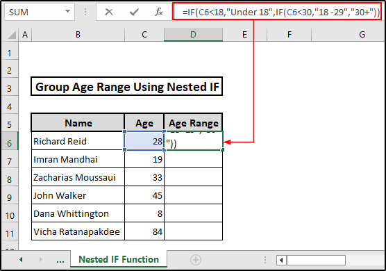
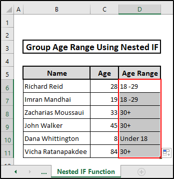
3. Excel Nested IF function to Group Age Range in Excel
You can also use the Nested IF function as an alternative to all other methods. This is relatively easy though. Suppose, we want to see in our dataset which ages are under 18, which are between 18 to 29, and which are above 30. Below we have demonstrated the steps where we have used the Nested IF function to do so.
⬇️⬇️ STEPS ⬇️⬇️
- First, select a cell where you want to specify the range. We have used cell D6 to show the range.
- In this selected cell insert the function below.
=IF(C6<18,"Under 18",IF(C6<30,"18 -29","30+"))
🔨 Formula Breakdown
IF(C6<18,”Under 18″,IF(C6<30,”18 -29″,”30+”))
👉 IF(C6<30,”18 -29″,”30+”), in this part of the function the cell C6 where the data is stored IF function runs a logic test, which means it compares the stored value with 30.
👉 After comparing, if this part is TRUE which means if the stored value in C6 is less than 30 then it will show the next statement, which is 18-29. If this is FALSE, or does not match the comparison, then it will show 30+.
👉 But this part of the function will run depending on the first part of the function.
👉 Here, in IF(C6<18,”Under 18″,IF(C6<30,”18 -29″,”30+”)), firstly the function will compare the value stored in cell C6 with 18. If this comparison is TRUE, then it will show the Under 18. Or, if not, then it will run the second part of the function, which is nested If portion discussed above.
- After that, press Enter and you will see the range where the age belongs.
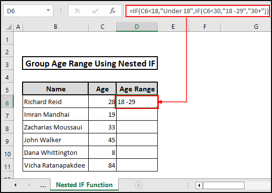
In this case, you can see, it is shown that the age 28 belongs to the range 18-29.
- Finally, use the Fill Handle icon to fill up the remaining cells.
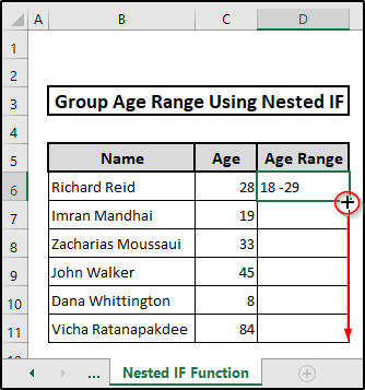
- The function will be inserted in every cell with modification due to this.
📝 Takeaways from This Article
📌 You have learned how to group age ranges using the VLOOKUP function, step by step.
📌 Besides this, you can now also group age ranges even without the VLOOKUP function.
📌 As an alternate you will gain an idea about the use of Pivot Table, IF, INDEX, and MATCH functions.
Conclusion
VLOOKUP function is one of the easiest ways to group age ranges in Excel. If you can use it correctly then you may be able to handle even a large dataset very effectively. Please leave a comment if you have any suggestions or questions. Don’t forget to visit our ExcelDen page to enhance your Excel-related knowledge.
Related Articles
- 4 Approaches to Capitalize All Letters in Excel Without Formula
- 7 Ways to Calculate Average Attendance with Formula in Excel
- 6 Quick Ways to Create Dynamic List from Table in Excel
- 11 Examples to Do SUMIF in Date Range of Month and Year
- 7 Quick Ways to Calculate Average Percentage Increase in Excel


