In this lesson, I’ll demonstrate 7 effective approaches on how to use VLOOKUP to compare two lists. However, these techniques will enable you to solve the problems that led you here. You will master several crucial Excel features and functions during this article, which will come in extremely handy for any assignment using Excel.
📁 Download Excel File
The sample worksheet that was used during the discussion is available to download for free right here.
Overview of VLOOKUP
We use VLOOKUP function in Excel when a table or a range by row has to be searched for certain problems.
The syntax for VLOOKUP is like the following box.
VLOOKUP(lookup value, table array, col index-num, [range lookup])
lookup value – what you’re attempting to find
table array – where to search for it
col_index num – the range’s column number that contains the value to return
[range lookup] – return either an Approximate or Exact match. Also indicated by 1 or TRUE and 2 or FALSE.
This function is handy for any kind of problem that has to do with anything like searching for values in a certain area. This is a function that is most frequently used with the combination of other functions to create formulas effectively.
📕 Read More: 2 Ways to Use VLOOKUP Function with Two Lookup Values
Learn to Use VLOOKUP to Compare Two Lists with These 7 Methods
Here we have two lists of the products of two different shops. We are going to compare them in this article.
1. Using VLOOKUP Function to Return Common Values
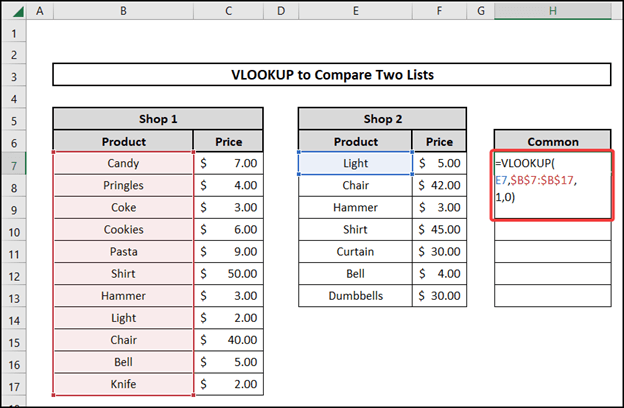
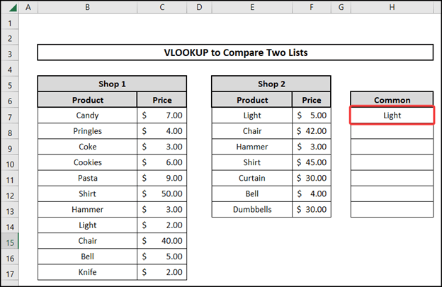
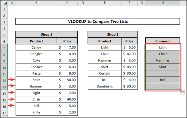
Here we have the datasheet for 2 shops and their products with prices. For instance, we are going to use VLOOKUP Function to determine the similarities here.
⬇️⬇️ STEPS ⬇️⬇️
- First, choose a cell you want to compare the two lists into and copy the following formula.
=VLOOKUP(E7,$B$7:$B$17,1,0)
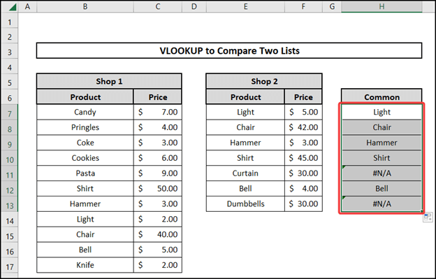
- After that, press Enter and copy down the formula for the results.
📕 Read More: 7 Ways to Use VLOOKUP to Compare Two Lists
2. Combining with IFERROR
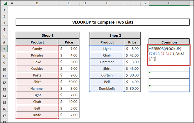
Here we will be combining VLOOKUP with IFERROR function. The IFERROR function delivers the value you provide if a formula evaluates to an error; else, it delivers the formula’s outcome. Now we are going to find the similarities between the two lists using this combination.
⬇️⬇️ STEPS ⬇️⬇️
- Select a cell and copy down the following formula.
=IFERROR(VLOOKUP(E7:E13,B7:B17,1,FALSE),””)
🔨 Formula Breakdown
👉 VLOOKUP(E7:E13,B7:B17,1,FALSE)
It looks for the value E7:E13 in the range B7:B17. 1 represents the column number of the range and FALSE refers to the exact value.
👉 IFERROR(VLOOKUP(E7:E13,B7:B17,1,FALSE),””)
The part says if the value is there show Value and if not, show nothing.
- Press Enter to see the results.

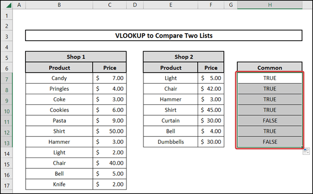
3. Applying NOT with VLOOKUP Function for Boolean Output
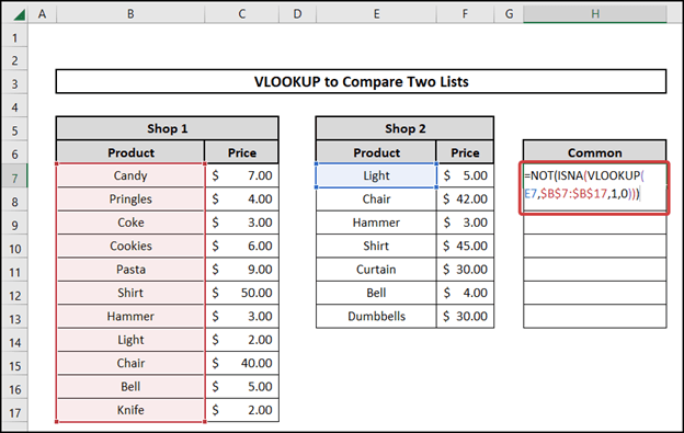
In this part we have the datasheet for 2 shops and their products with prices. We are going to use ISNA, VLOOKUP, and NOT Functions to determine the similarities here.
⬇️⬇️ STEPS ⬇️⬇️
- First, choose a cell you want to compare the two lists into and copy the following formula.
=NOT(ISNA(VLOOKUP(E7,$B$7:$B$17,1,0)))
🔨 Formula Breakdown
👉 VLOOKUP(E7,$B$7:$B$17,1,0)
It looks for the value E7 in the $B$7:$B$17 range. 1 represents the column number of the range and 0 refers to the exact value.
👉 ISNA(VLOOKUP(E7,$B$7:$B$17,1,0))
The ISNA function allows for smooth comparisons and assists in finding cells with a #N/A errors.
👉 NOT(ISNA(VLOOKUP(E7,$B$7:$B$17,1,0)))
The part says if the value is there show True and if not show FALSE.
- Press Enter and copy the formula down for the results.
📕 Read More: 6 Solutions If VLOOKUP Returns #N/A When Match Exists in Excel
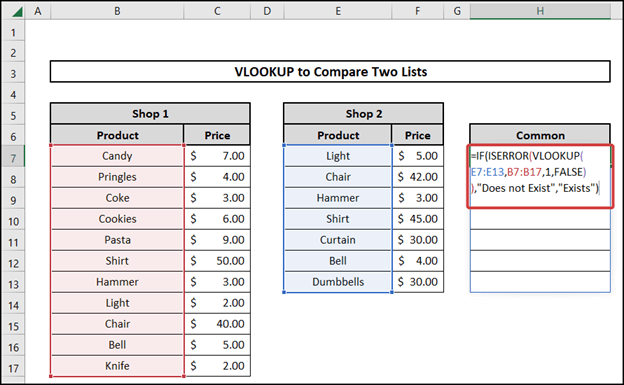
4. Combining ISERROR with VLOOKUP
In this part we have the datasheet for 2 shops and their products with prices. We are going to use IF, ISERROR, and VLOOKUP Functions to determine the similarities here. We are working with products of Shop 2 and checking whether they exist in Shop 1 or not.
⬇️⬇️ STEPS ⬇️⬇️
- First choose a cell you want to compare the two lists into and copy the following formula.
=IF(ISERROR(VLOOKUP(E7:E13,B7:B17,1,FALSE)),”Does not Exist”,”Exists”)
🔨 Formula Breakdown
👉 VLOOKUP(E7:E13,B7:B17,1,FALSE)
It looks for the values of E7:E13 in the range B7:B17. 1 represents the column number of the range and FALSE refers to the exact value.
👉 ISERROR(VLOOKUP(E7:E13,B7:B17,1,FALSE))
The ISERROR function determines if a mathematical phrase indicates an error or not.
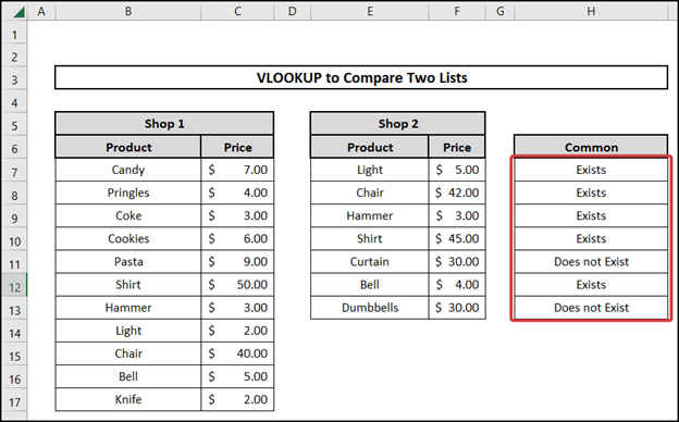
👉 IF(ISERROR(VLOOKUP(E7:E13,B7:B17,1,FALSE)),”Does not Exist”,”Exists”)
The part says if the value is there show Exists and if not show the Does not Exist.
- Press Enter to get all the answers.
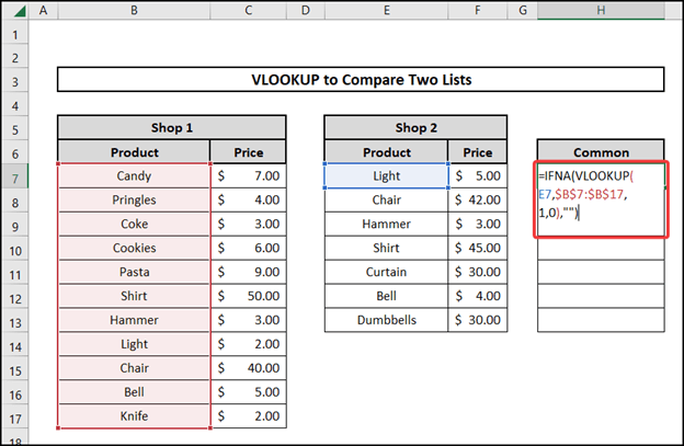
5. Applying IFNA with VLOOKUP Function for Boolean Output
Here we have the datasheet for 2 shops and their products with prices. We are going to use VLOOKUP and IFNA Functions to determine the similarities here.
⬇️⬇️ STEPS ⬇️⬇️
- First choose a cell you want to compare the two lists into and copy the following formula.
=IFNA(VLOOKUP(E7,$B$7:$B$17,1,0),””)
🔨 Formula Breakdown
👉 VLOOKUP(E7,$B$7:$B$17,1,0)
It looks for the value E7 in the $B$7:$B$17 range. 1 represents the column number of the range and 0 refers to the exact value.
👉 IFNA(VLOOKUP(E7,$B$7:$B$17,1,0),””)
This part says if the value is there show the Value and otherwise show nothing.
- Press Enter to see the result.
- Copy down the formula for the whole column.
📕 Read More: 8 Ways to VLOOKUP to Return Multiple Values Vertically in Excel
6. Combining with IF for Custom Output
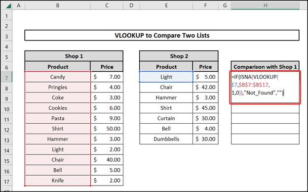
Here we are going to detect which values of Shop 2 are not common. Therefore, we are using IF, ISNA, and VLOOKUP functions here.
⬇️⬇️ STEPS ⬇️⬇️
- First, Select a cell and copy the following formula.
=IF(ISNA(VLOOKUP(E7,$B$7:$B$17,1,0)),”Not_Found”,””)
🔨 Formula Breakdown
👉 VLOOKUP(E7,$B$7:$B$17,1,0)
It looks for the value E7 in the $B$7:$B$17 range. 1 represents the column number of range and 0 refers to the exact value.
👉 ISNA(VLOOKUP(E7,$B$7:$B$17,1,0))
The ISNA function allows for smooth comparisons and assists in finding cells with a #N/A errors.
👉 IF(ISNA(VLOOKUP(E7,$B$7:$B$17,1,0)),”Not_Found”,””)
The part says if the value is there show nothing and if not show Not_Found.
- Press Enter and copy down the formula for the total result.
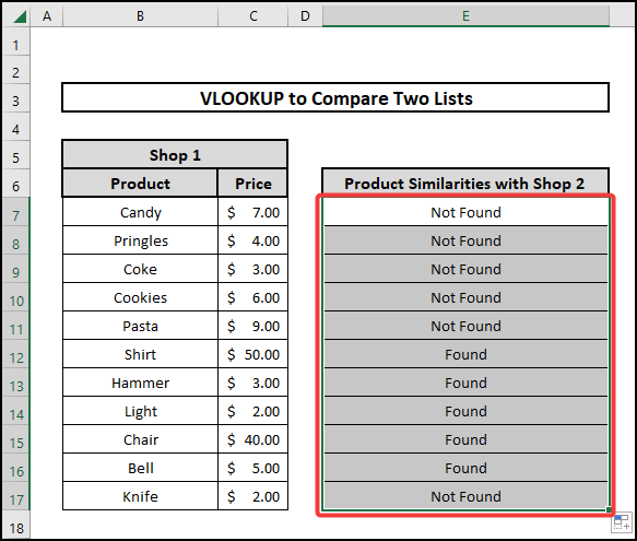
7. Compare Two Columns in Different Worksheets Using VLOOKUP
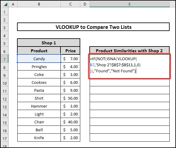
In this paragraph we have a dataset in two different Sheets. We are going to compare them in this section using different functions like the previous methods which are VLOOKUP, ISNA, NOT, and IF functions.
⬇️⬇️ STEPS ⬇️⬇️
- First copy the following formula, be careful as there is a part that says the sheet’s name in the formula.
=IF(NOT(ISNA(VLOOKUP(B7,’Shop 2′!$B$7:$B$13,1,0))),”Found”,”Not Found”)
🔨 Formula Breakdown
👉 VLOOKUP(B7,’Shop 2′!$B$7:$B$13,1,0)
It looks for the value B7 of the sheet Shop 1 in the $B$7:$B$13 range of sheet Shop 2. 1 represents the column number of the range and 0 refers to the exact value.
👉 ISNA(VLOOKUP(B7,’Shop 2′!$B$7:$B$13,1,0))
The ISNA function allows for smooth comparisons and assists in finding cells with a #N/A errors.
👉 IF(NOT(ISNA(VLOOKUP(B7,’Shop 2′!$B$7:$B$13,1,0))),”Found”,”Not Found”)
The part says if the value is there show Found nothing and if not show Not Found.
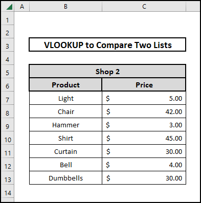
In addition this is the Other Sheet Data here down below which has the name Shop 2.
- After that, press Enter and copy down to check the similarities between two different sheets.
📕 Read More: VLOOKUP to Find Duplicates in Two Columns in Excel
📄 Important Notes
🖊️ Be careful while using the code as there are a lot of terms and if you lose concentration the code may be incorrect.
🖊️ Use shortcuts to reduce time.
🖊️ While writing formulas carefully see the suggestions and don’t forget the commas and parentheses.
🖊️ However use F4 for defining absolute value in the formula.
🖊️ Check if anything in the formula is in italic form or not.
📝 Takeaways from This Article
📌 Use of VLOOKUP, ISNA, IFNA, IF, and NOT functions.
📌 How to VLOOKUP to compare two lists both in the same sheet and different sheets.
📌 Determining similarities.
📌 In addition, Obtaining dissimilarities.
Conclusion
Firstly I hope you were able to use the techniques I demonstrated in this VLOOKUP to Compare Two Lists. However as you can see, there are a lot of options on how to do this. Decide deliberately on the approach that best addresses your circumstance therefore, I advise repeating the steps if you become confused in any of the steps if you get stuck. Practice on your own after taking a look at VLOOKUP to Compare Two Lists Excel file in the practice workbook as I’ve provided above because practice makes a man perfect. Above all I earnestly hope you can use it. In conclusion, Please share your experience with us in the comment box about how your experience was throughout the article and what we need to improve or add to make things better for you folks. Moreover if you have any problem regarding Excel spit it in the comment box. The Excelden crew is always available to answer your questions. Keep educating yourself by reading. For more Excel-related articles please visit our website Excelden.com.
Related Articles
- 3 Quick Ways to Vlookup and Return Multiple Values Horizontally
- 5 Ways to Extract Filtered Data into Another Excel Sheet
- Find MAX of Multiple Values Using VLOOKUP Function in Excel
- 5 Examples to Use IF and VLOOKUP as Nested Function in Excel


