What Is Table Array in VLOOKUP in Excel?

In Microsoft Excel, a table array is one of the required arguments for all lookup functions. We have described what table array is in the VLOOKUP function in Excel by demonstrating 5 examples in this article.

Contents hide

📁 Download Excel File

What Is VLOOKUP Function and Table Array in Excel?

Learn What Table Array Is in VLOOKUP Function in Excel with These 5 Examples

1. Applying VLOOKUP in Same Sheet

2. Employing VLOOKUP in Another Sheet

3. Using VLOOKUP for Variable Table Array

4. Using User-Defined Names

5. Creating Table

Solution: #N/A Error for Not Locking Table Reference in VLOOKUP

Advantages and Disadvantages of Table Array in VLOOKUP Function

📄 Important Notes

📝 Takeaways from This Article

Conclusion

📁 Download Excel File

You can download the Excel file used for the demonstration from the link below.

Table Array in VLOOKUP.xlsx

What Is VLOOKUP Function and Table Array in Excel?

The VLOOKUP Function:

The VLOOKUP function searches for a value by row in a range or an array and returns the exact or approximate match. So, in its most basic form, this function says:

=VLOOKUP(the value to look for, where to look for, which column to look for, want an approximate match or exact match)

Now, let us look at the syntax of the VLOOKUP function:

VLOOKUP (lookup_value, table_array, col_index_num, [range_lookup])

So, we need four pieces of information to build VLOOKUP syntax:

Lookup value: The value you want to look up. It can be a text, number, or cell reference.

Table Array: The range or table reference contains the value you want to return.

Column index number: This is the index number of columns in the table array, which contains the value to return.

Range lookup: It is a logical value that represents if you want an exact or approximate match. For an approximate match, the input is 1 or TRUE, and for an exact match is 0 or FALSE.

The Table Array:

At this point, let us look a bit more into the Table Array argument.

An argument is a mandatory piece of information to run any function, and every lookup function requires a cell range where it looks for the desired value, which is a table array argument. The first argument for lookup functions is always the value to look up, and the table array is always the second.

Excel takes input for this argument in diverse ways, such as a table, a named range, or names instead of cell references. However, the lookup value must be in the first column of the cell range. Moreover, the return value needed to be included in the range.

Now, let us see some examples of applying a table array in VLOOKUP function.

Learn What Table Array Is in VLOOKUP Function in Excel with These 5 Examples

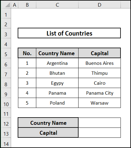
We used a dataset containing some countries’ names and capitals to illustrate the examples. We will look up countries’ names to return their capital names. Hence, we will demonstrate how to apply table array differently in VLOOKUP function in Excel with this dataset.

Approach 1

1. Applying VLOOKUP in Same Sheet

In this first example, we will demonstrate the simplest use of table array in VLOOKUP function. Let us go through the steps to apply this function.

⬇️⬇️ STEPS ⬇️⬇️

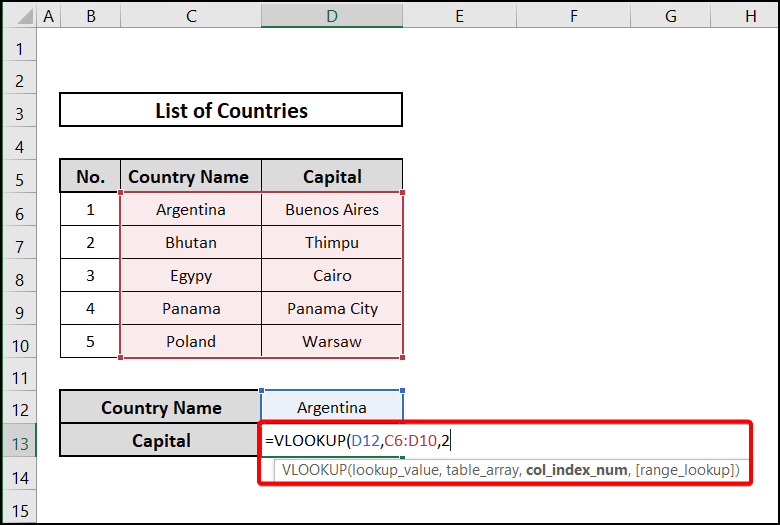
First, select cell D13 and type the VLOOKUP.

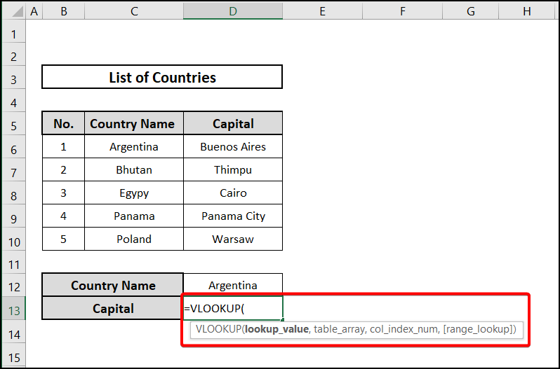
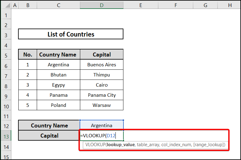
Here, the lookup value is Argentina which is in cell D12. So, type D12 first into the function.

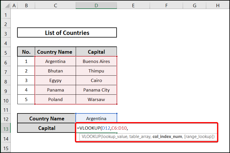
Next, enter C6:D10 as a table array. Here, column C contains the lookup value, and column D contains the return value.

After that, type 2 as the column index number because the second column of the table array contains the return value.

Then, select FALSE as range lookup for the exact match, close the bracket, and hit Enter.

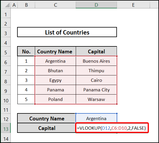
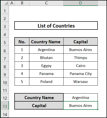
Lastly, the desired value will be returned in cell D13.

Approach 2

2. Employing VLOOKUP in Another Sheet

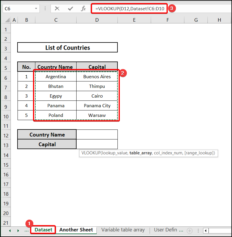
We will show in this example how to use a table array from another sheet in VLOOKUP function in Excel. So, we named our current worksheet Another Sheet and will enter the table array from the Dataset worksheet. So, let us see the steps.

⬇️⬇️ STEPS ⬇️⬇️

First, select cell D13 and type the VLOOKUP.
Here, the lookup value is Egypt which is in cell D12. So, type D12 first into the function.

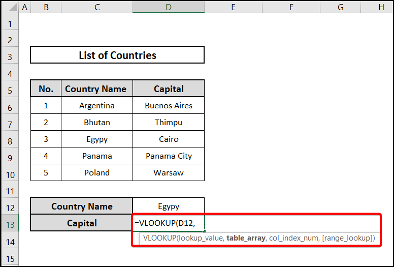
Next, to enter the table array click on Dataset worksheet and select C6:D10, and it will be inserted in our current worksheet as Dataset!C6:D10. Here, column C contains the lookup value, and column D contains the return value.

After that, type 2 as the column index number because the second column of the table array contains the return value, and then select FALSE as range lookup for the exact match, close the bracket, and hit Enter.

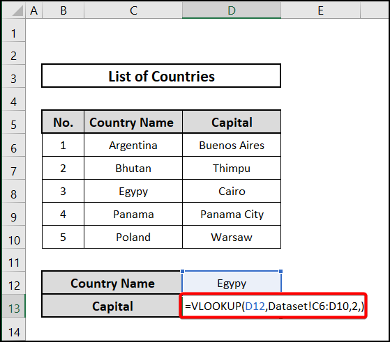
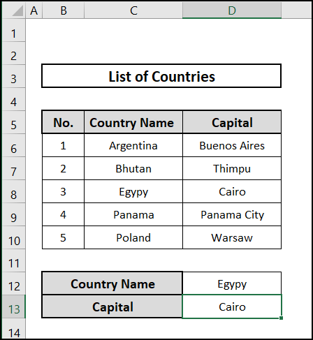
Lastly, the desired value will be returned in cell D13.

Approach 3

3. Using VLOOKUP for Variable Table Array

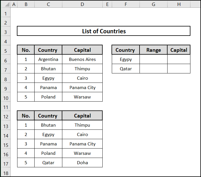
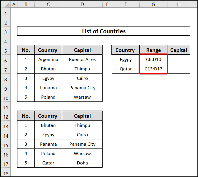
Now we will demonstrate in this example how to use a variable table array in VLOOKUP function in Excel. For that, we have two lists of the capitals of several countries.

Let us see the steps now.

⬇️⬇️ STEPS ⬇️⬇️

First, enter the array C6:D10 and C13:D17 in cells G6 and G7, which will be used as a table array.

Next, insert the formula in cell H6.

=VLOOKUP(F6,INDIRECT(G6),2,FALSE)

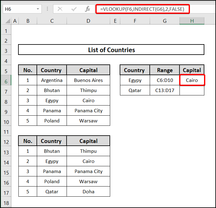
Here, the lookup value is in cell F6. Then, the INDIRECT function returns the value of cell G6 as a cell reference. 2 denotes the column number of the return value and FALSE is for an exact match.

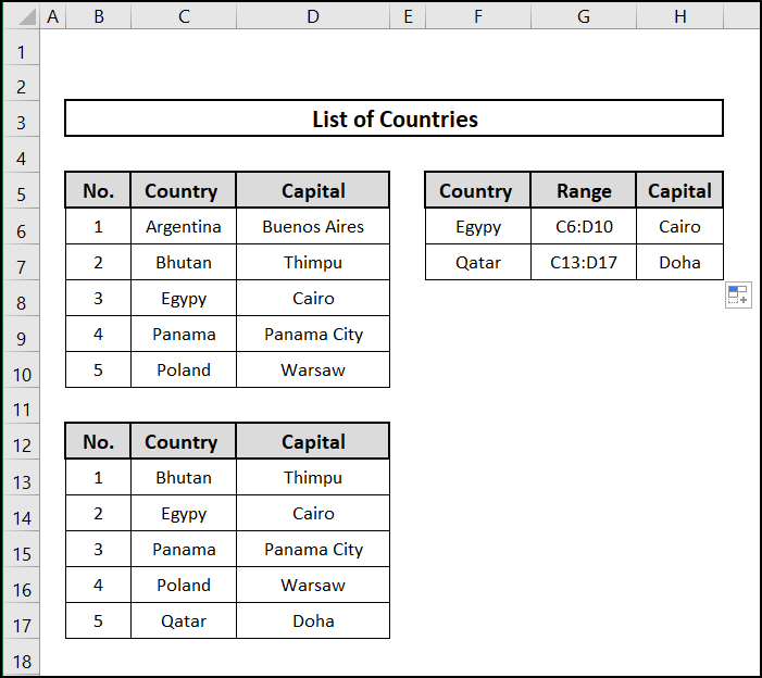
Lastly, drag the Fill Handle down and we will have the desired value returned in cells.

📕 Read More: 7 Ways to Use VLOOKUP to Compare Two Lists

Approach 4

4. Using User-Defined Names

In this example, we will use the user-defined name as a table array in VLOOKUP function in Excel. Let us go through the steps.

⬇️⬇️ STEPS ⬇️⬇️

At first, select the range C6:D10, and in the name box type Table and the name of this range as Table will be defined.

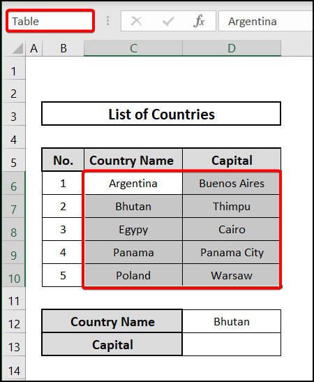
Now, insert the formula in cell D13 and have the desired outcome.

=VLOOKUP(D12,Table,2,FALSE)

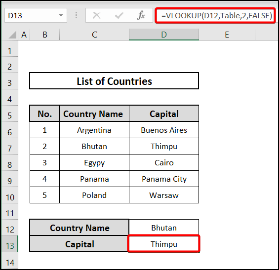
Here, the lookup value is in cell D12. Then, Table refers the cell references as table array. 2 denotes the column number of return value and FALSE is for an exact match.

Approach 5

5. Creating Table

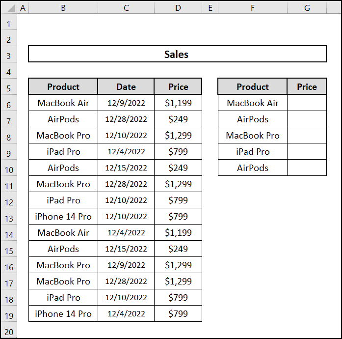
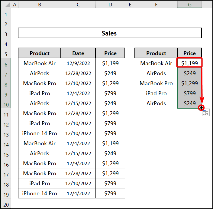
In this example, we will demonstrate using a table array in VLOOKUP function to create a table in Excel. To demonstrate this, we have a sales dataset containing the product name, selling date, and price of products. Now, we want to create a table with only the product name and price.

Let us go through the steps.

⬇️⬇️ STEPS ⬇️⬇️

At first, select cell G6, which will be the active cell. Now, click on the Insert Function option of the formula bar.

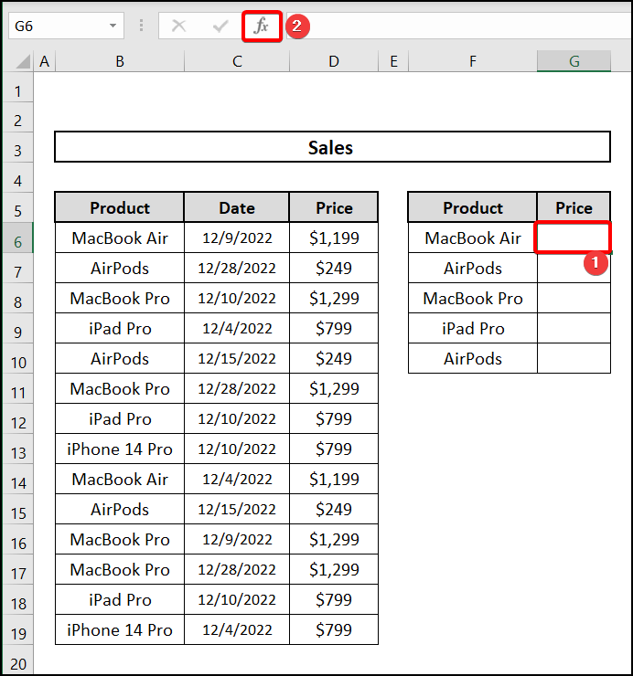
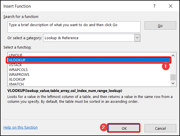
Then, the Insert Function box will appear. Select VLOOKUP from the Select a function option and click on OK.

After that, Function Arguments named box will pop up. There enter F6 as Lookup value, $B$6:$D$19 as Table array, 3 as Col index num, and False as Range lookup, and press OK.

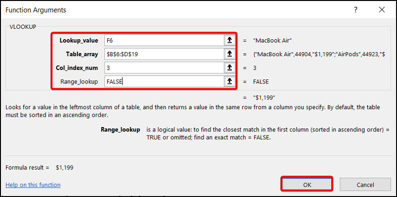
In cell G6, we will have the desired outcome. Now, drag the Fill handle down to Autofill the cells, and we will have the table.

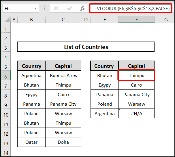
Solution: #N/A Error for Not Locking Table Reference in VLOOKUP

At times, #N/A or Value Not Available error might appear while using VLOOKUP function in multiple cells.

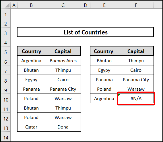
Here, this error is caused because the table reference is not locked in the function. As a result, when we auto filled down the rest of the cells with this formula, the table reference changed automatically, and the lookup value in cell E10 is not available in that range, thus showing an error.

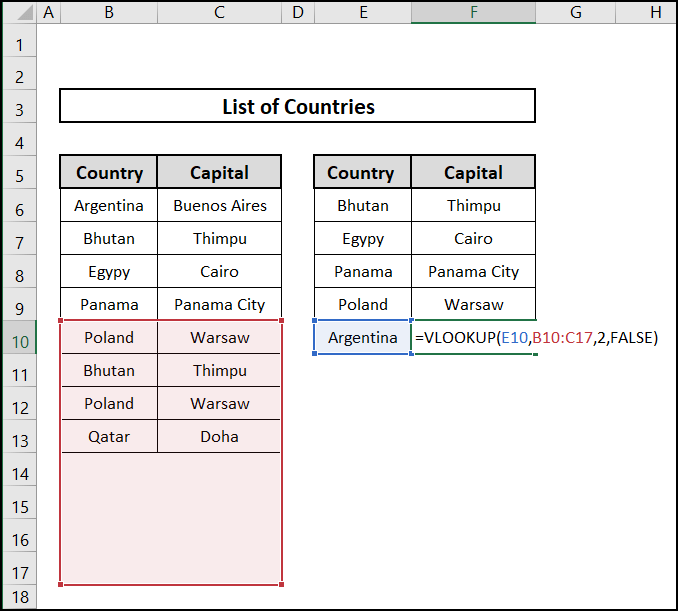
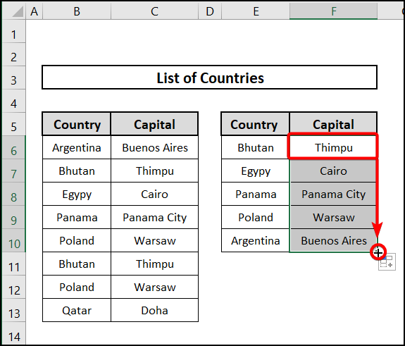
To solve this problem, select the cell reference of cell F6 on the formula bar and press F4, which will make the references absolute cell references and will get locked.

Now, if we autofill the other cells, the cell reference of the table array will not change, and there will be no error.

Advantages and Disadvantages of Table Array in VLOOKUP Function

A single table can be created from similar and co-related data.
Before applying the formula, we can name the table on cell range to keep the syntax small.
Any additional table arrays can be used for VLOOKUP.
If the data in tables are not co-related, then VLOOKUP is not useful.

📄 Important Notes

🖊️ Always ensure that the first column of table array contains the lookup value.

🖊️ This function will not work if the tables are not co-related.

📝 Takeaways from This Article

📌 This article described what table array is in VLOOKUP function with 5 examples.

📌 In the first example, we showed the simplest way of using table arrays in VLOOKUP function in Excel.

📌 Then, we demonstrated how to apply a table array from a different worksheet.

📌 After that, we applied a variable table array.

📌 Next, we defined a name for the table array in VLOOKUP function.

📌 Finally, we showed how to create a table using table array in VLOOKUP function in Excel.

Conclusion

This article has described what table array is in VLOOKUP function in Excel with 5 examples. All these formulas are incredibly effective and simple to use. We hope this article helps you. Please leave a remark if you have any queries. The author will do their best to find an appropriate answer.

For more guides like this, visit Excelden.com.