In this lesson, I’ll demonstrate 11 effective approaches so that you can use Excel to extract data from table based on multiple criteria including some other problems related to this one. These techniques will enable you to solve the problem that led you here. You will master several crucial Excel features and functions during this article, which will come in extremely handy for any assignment using Excel.
📁 Download Excel File
The sample worksheet that was used during the discussion is available to download for free right here.
Learn to Extract Data from Table Based on Multiple Criteria in Excel Using These 11 Methods
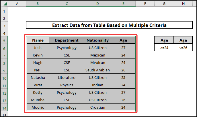
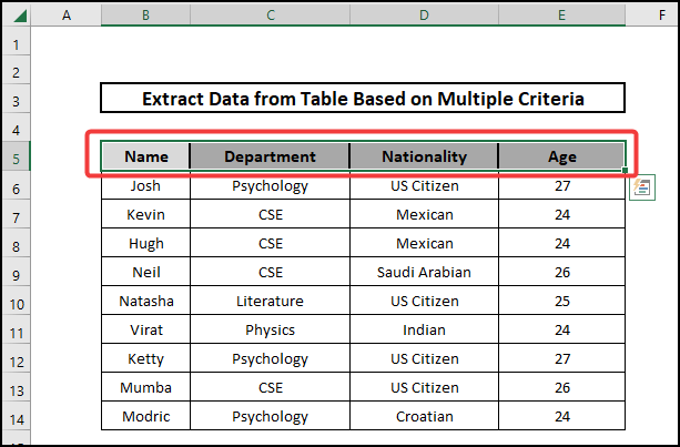
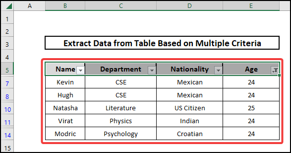
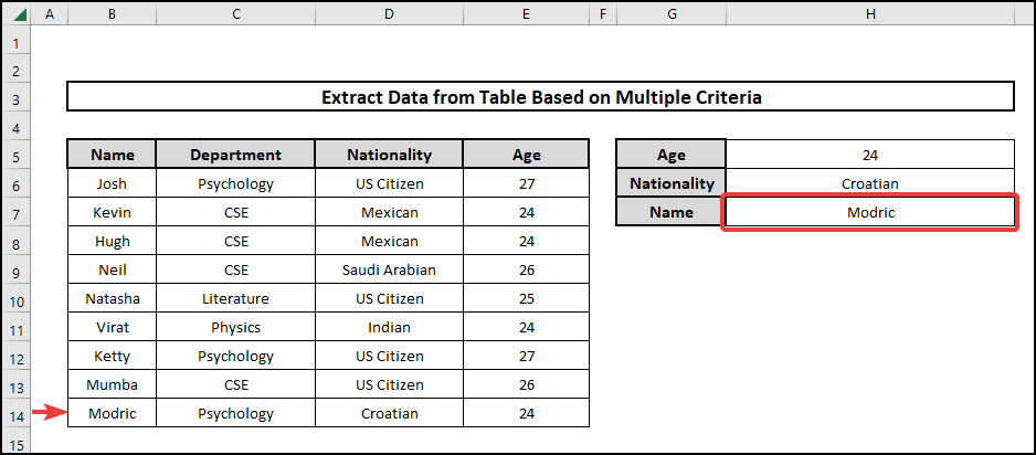
Here we have the dataset of students of different departments, Age and nationality. We will demonstrate how to extract data from this table based on multiple criteria using different functions.
1. Advanced Filter Command Tool
The Filter Command Tool is a very handy feature in Excel to act according to certain criteria. Here we have a dataset of students from different regions, different ages, and departments. We are going to extract data from the table based on the ages that are between 24 to 26. For this, we have to assign two new columns with those criteria.
⬇️⬇️ STEPS ⬇️⬇️
- Firstly, we will select the whole table using the mouse cursor.
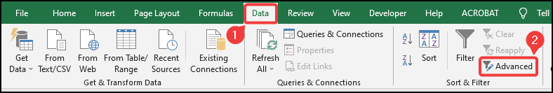
- After that, use the Advanced Filter option from the Data tab of the Ribbon.
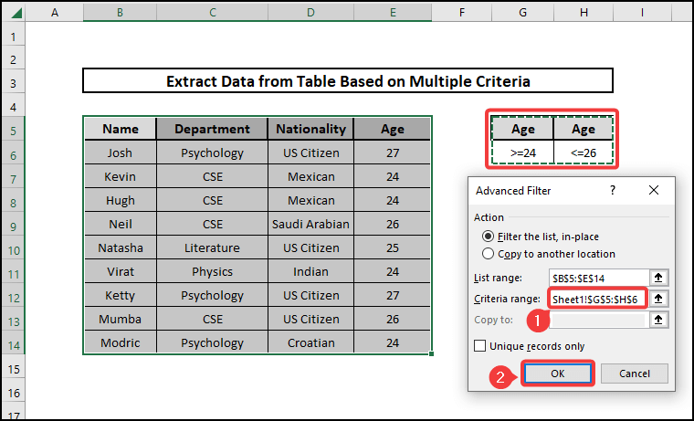
- Then a new window will pop up. Select the criteria range using the mouse cursor like the picture below and press OK.
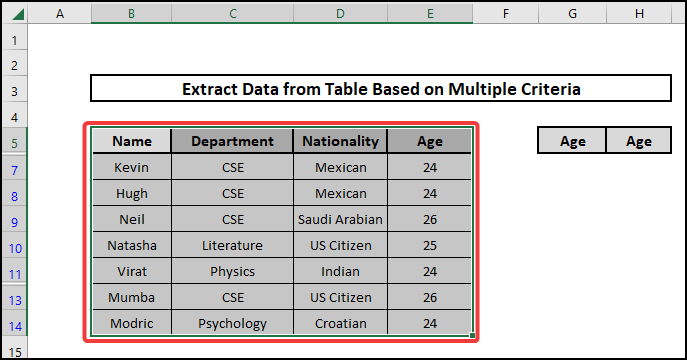
- Now in conclusion you can see we have successfully filtered the table keeping the data for only people between the age of 24 to 26.
📕 Read More: Pull Same Cell from Multiple Sheets into Master Column
2. Using Filter Tool
Now we will be using the Filter Tool from the ribbon to extract data from the table based on multiple criteria in Excel.
⬇️⬇️ STEPS ⬇️⬇️
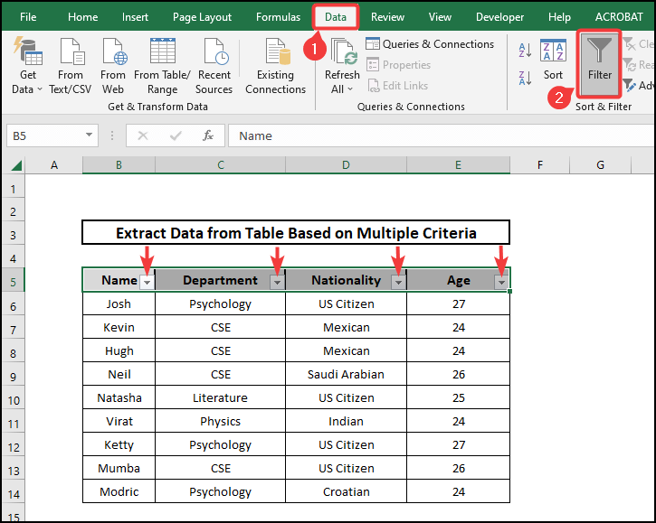
- Initially, we’ll merely choose the dataset’s headline.
- After that, go to Data from the ribbon and select the Filter You’ll see the headlines will have dropdown buttons like the picture below.
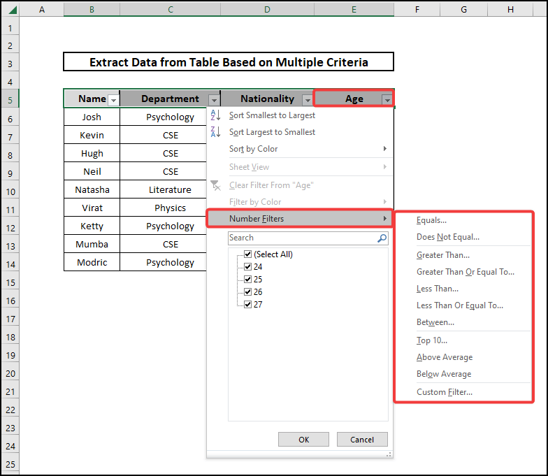
- Now as you click on any of the downward-facing buttons, more options will pop up. You can go to Number Filters to get options to filter the data as you want. You can play around with it as you can see there are too many options.
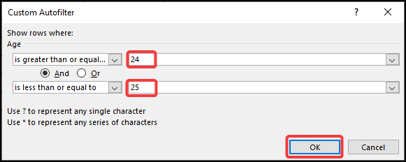
- For instance, we are demonstrating how to filter data of people between the age of 24 to 25. So we selected the Between option from the Number Filters option and a new window appeared like the picture below. We are applying the criteria range 24 to 25.
- Lastly, here is the result.
📕 Read More: 6 Ways to Extract Data from Excel Based on Criteria
3. Converting into Tables
We can use the Insert Table option to extract data from an existing table.
⬇️⬇️ STEPS ⬇️⬇️
- First, go to the Table option from the Insert tab from the ribbon.

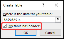
- After that, a dialogue box will appear to select the dataset you have here we are selecting B5:E14. Make sure My table has headers option ticked. Press OK.
- You’ll see dropdown buttons like the Filter Command method.
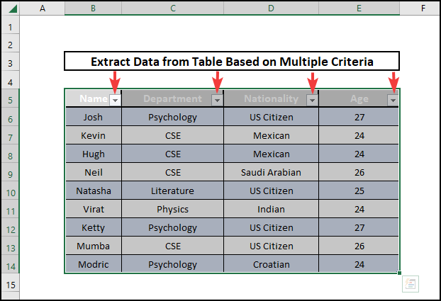
- Now using the dropdown buttons you can filter the dataset as you want like the Filter Tool method.
📕 Read More: 5 Ways to Extract Filtered Data into Another Excel Sheet
4. Utilizing INDEX-MATCH Formula
In this case, we’ll use the INDEX and MATCH functions to retrieve data based on a variety of criteria creating an array formula.
⬇️⬇️ STEPS ⬇️⬇️
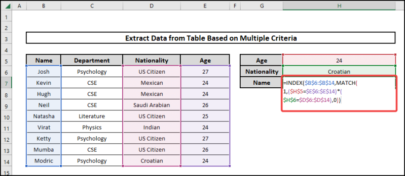
- First, we have to create cells that define our criteria. Then we need to apply the combined array formula written down below for this problem.
=INDEX($B$6:$B$14,MATCH(1,($H$5=$E$6:$E$14)*($H$6=$D$6:$D$14),0))
🔨 Formula Breakdown
👉 MATCH(1,($H$5=$E$6:$E$14)*($H$6=$D$6:$D$14),0)
Here a lookup value’s location in a range is found using the MATCH function. Lookup value is 1 lookup array is ($H$5=$E$6:$E$14)*($H$6=$D$6:$D$14) and it means the value 24 in E6:E14 and Croatian in D6:D14. Match type 0 refers to the exact match.
👉 INDEX($B$6:$B$14,MATCH(1,($H$5=$E$6:$E$14)*($H$6=$D$6:$D$14),0))
The value at a specific place in a range is returned by the INDEX function. $B$6:$B$14 is the array here for INDEX function.
Output: Modric
👉 Explanation:Modric is the Name based on the Nationality and Age.
- Now press Ctrl+Shift+Enter if you’re not a Microsoft 365 user or press Enter for results.
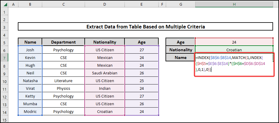
5. INDEX-MATCH Formula for Non-Array
This section uses the combination of INDEX and MATCH functions to create a non-array formula to extract data from tables based on multiple criteria.
⬇️⬇️ STEPS ⬇️⬇️
- First copy down the following non-array formula.
=INDEX($B$6:$B$14,MATCH(1,INDEX(($H$5=$E$6:$E$14)*($H$6=$D$6:$D$14),0,1),0))
🔨 Formula Breakdown
👉 MATCH(1,INDEX(($H$5=$E$6:$E$14)*($H$6=$D$6:$D$14),0,1),0)
Here a lookup value’s location in a range is found using the MATCH function. ($H$5=$E$6:$E$14)*($H$6=$D$6:$D$14) means both values which are 24 in E6:E14 and Croatian in D6:D14 respectively.
👉 INDEX($B$6:$B$14,MATCH(1,INDEX(($H$5=$E$6:$E$14)*($H$6=$D$6:$D$14),0,1),0))
The value at a specific place in a range is returned by the INDEX function.
Output: Modric
👉 Explanation:Modric is the Name based on the Nationality and Age.
- Press Enter to get the results.
📕 Read More: 4 Ways to Pull Values in Excel from Another Worksheet
6. Employing LOOKUP Function to Extract Data from Table
Here we are going to use the LOOKUP function to extract data from tables based on multiple criteria in Excel.
⬇️⬇️ STEPS ⬇️⬇️
- At the start, copy the following formula for searching the specific data we are looking for.
=LOOKUP(1,1/($E$6:$E$14=$H$5)/($D$6:$D$14=$H$6),($B$6:$B$14))
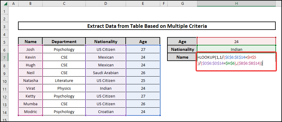
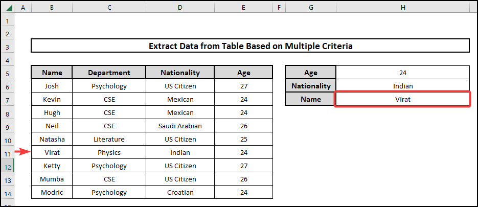
- Press Enter for the result.
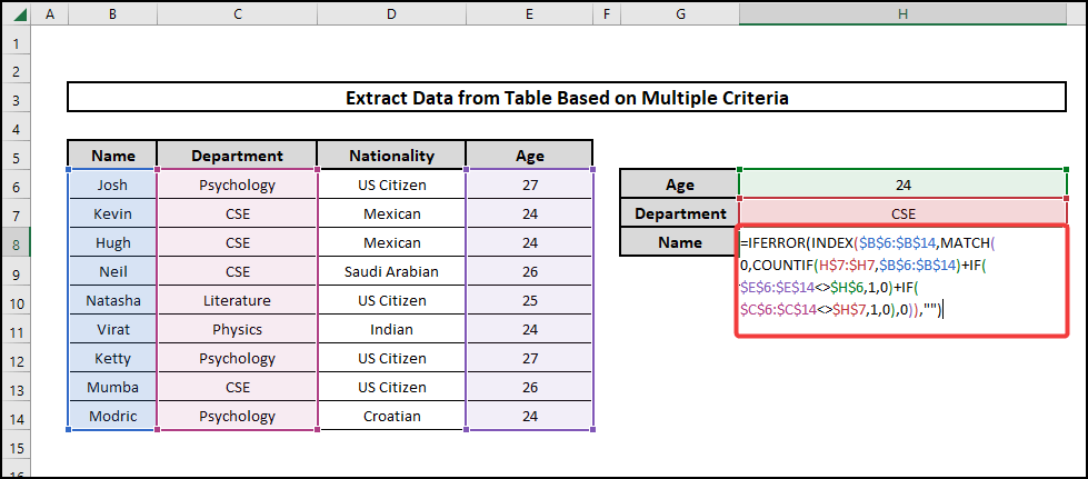
7. Combining INDEX-MATCH with COUNTIF
This is for multiple results against given criteria using IFERROR, INDEX, MATCH, and COUNTIF to create an array.
⬇️⬇️ STEPS ⬇️⬇️
- First copy down the following formula.
=IFERROR(INDEX($B$6:$B$14,MATCH(0,COUNTIF(H7:$H$7,$B$6:$B$14)+IF($E$6:$E$14<>$H$6,1,0)+IF($C$6:$C$14<>$H$7,1,0),0)),””)
🔨 Formula Breakdown
👉 INDEX($B$6:$B$14,MATCH(0,COUNTIF(H7:$H$7,$B$6:$B$14)+IF($E$6:$E$14<>$H$6,1,0)+IF($C$6:$C$14<>$H$7,1,0),0))
The value at a specific place in a range is returned by the INDEX function.
👉 COUNTIF(H7:$H$7,$B$6:$B$14)
Cells in a range that satisfy a single condition are counted using the COUNTIF function.
👉 MATCH(0,COUNTIF(H7:$H$7,$B$6:$B$14)+IF($E$6:$E$14<>$H$6,1,0)+IF($C$6:$C$14<>$H$7,1,0),0)
Here a lookup value’s location in a range is found using the MATCH function.
👉 IFERROR(INDEX($B$6:$B$14,MATCH(0,COUNTIF(H7:$H$7,$B$6:$B$14)+IF($E$6:$E$14<>$H$6,1,0)+IF($C$6:$C$14<>$H$7,1,0),0)),””)
In cases when there is a formula error, the IFERROR function returns a cell.
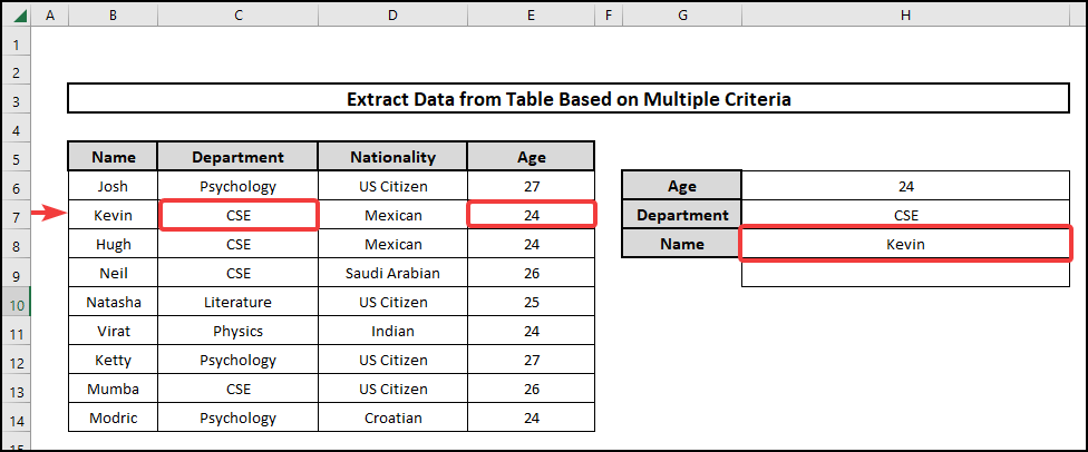
Output: Kevin
👉 Explanation: Kevin is the Name of the student based on the Department and Age.
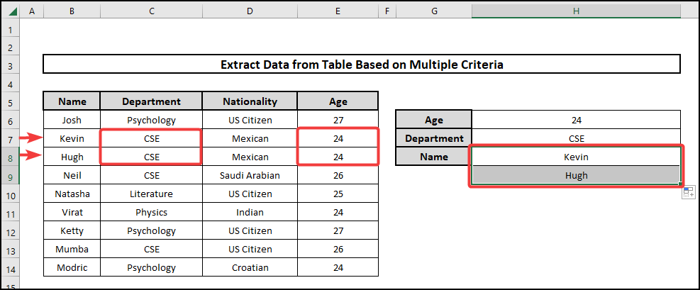
- Press Ctrl+Shift+Enter if you’re not a Microsoft 365 user or press Enter for results.
- Now Copy down the formula for other results.
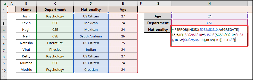
8. Combining INDEX and AGGREGATE for Multiple Answers
Here we will be Using a bunch of functions which includes IFERROR, INDEX, AGGREGATE, and ROW. Remember this formula needs the dataset to start from ROW 1.
⬇️⬇️ STEPS ⬇️⬇️
- Copy down the following formula.
=IFERROR(INDEX($D$2:$D$10,AGGREGATE(15,6,IF(($E$2:$E$10=$H$2)*($C$2:$C$10=$H$3), ROW($D$2:$D$10)),ROW(1:1))-1,1),””)
🔨 Formula Breakdown
👉 ROW($D$2:$D$10)
The row number of specific cells is obtained via the ROW function.
👉 IF(($E$2:$E$10=$H$2)*($C$2:$C$10=$H$3), ROW($D$2:$D$10))
The IF function compares a supplied value to an anticipated value logically.
👉 AGGREGATE(15,6,IF(($E$2:$E$10=$H$2)*($C$2:$C$10=$H$3), ROW($D$2:$D$10)),ROW(1:1))
When used on a dataset, the AGGREGATE function returns an aggregate.
👉 INDEX($D$2:$D$10,AGGREGATE(15,6,IF(($E$2:$E$10=$H$2)*($C$2:$C$10=$H$3), ROW($D$2:$D$10)),ROW(1:1))-1,1)
The value at a specific place in a range is returned by the INDEX function.
👉 IFERROR(INDEX($D$2:$D$10,AGGREGATE(15,6,IF(($E$2:$E$10=$H$2)*($C$2:$C$10=$H$3), ROW($D$2:$D$10)),ROW(1:1))-1,1),””)
In cases when there is a formula error, the IFERROR function returns a cell.
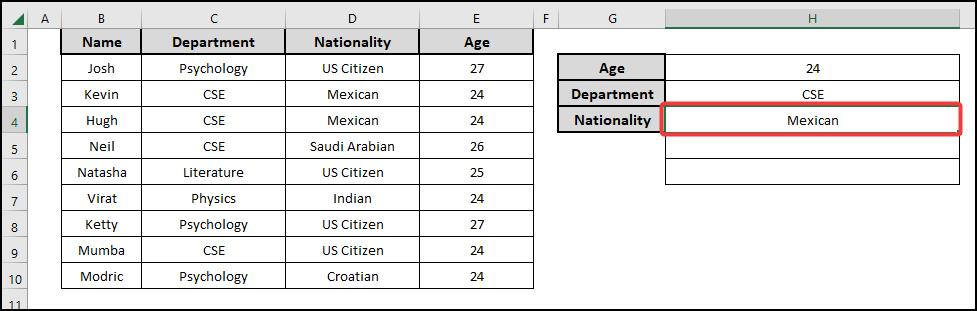
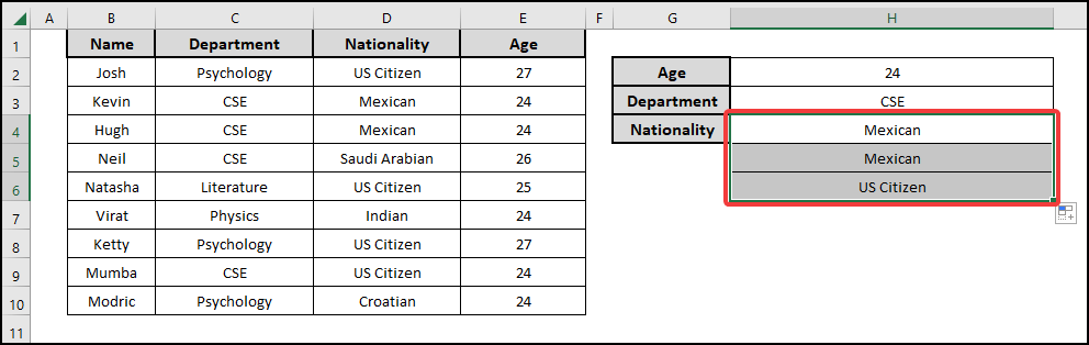
Output: Mexican
👉 Explanation: Mexican is the Nationality of the students based on the Department and Age.
- Press Ctrl+Shift+Enter if you’re not a Microsoft 365 user or press Enter for results.
- Copy down the formula for the remaining answers.
9. Using FILTER Function
The following paragraph will instruct you to use the FILTER function to extract data from tables based on multiple criteria.
⬇️⬇️ STEPS ⬇️⬇️
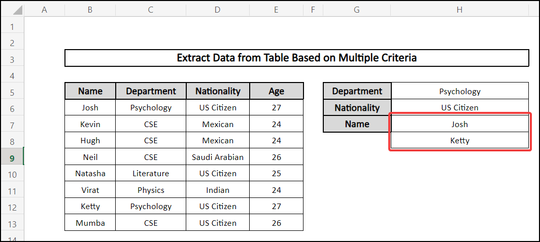
- Copy down the following formula. Keep in mind that this FILTER Function works on Microsoft 365 only.
=FILTER(B6:B13,(H5=C6:C13)*(H6=D6:D13))
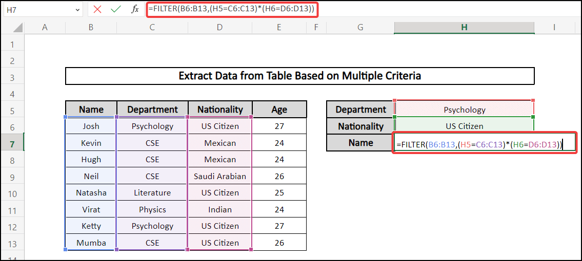
- After that press Enter and you will get all the answers.
10. Utilizing SUM Function
Using the SUM function here to determine the age of a specific person from a dataset which is a Numerical Value.
⬇️⬇️ STEPS ⬇️⬇️
- Copy the following formula down.
=SUM((B6:B14=H6)*(C6:C14=H7)*(E6:E14))
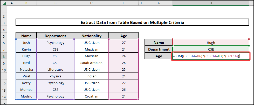
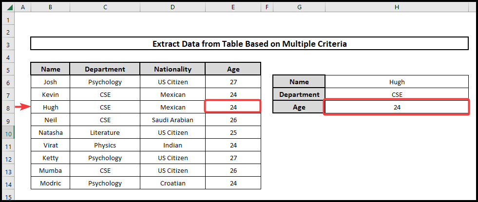
- Press Enter for the result. Most importantly remember this function works for finding Numerical Numbers.
11. Utilizing SUMIFS Function
Here we will be using the SUMIFS function to determine the age of a specific person from a dataset which is a Numerical Value.
⬇️⬇️ STEPS ⬇️⬇️
- Select and copy the following formula of the SUMIFS function.
=SUMIFS(E6:E14,D6:D14,H6,B6:B14,H7)
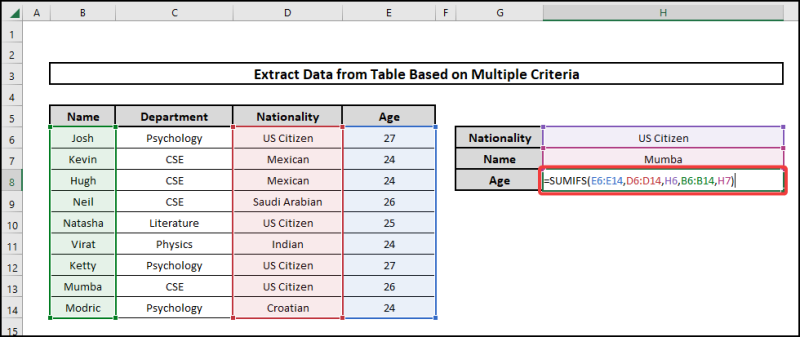
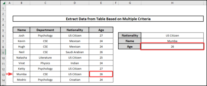
- Press Enter to get the result. Remember this function also works for Numerical Values.
📄 Important Notes
🖊️ Be careful while using the code as there are a lot of terms and if you lose concentration the code may be incorrect.
🖊️ In addition Use shortcuts to reduce time.
🖊️ Use Ctrl+Shift+Enter for arrays if you are not using Microsoft 365.
🖊️ While writing formulas carefully see the suggestions and don’t forget the commas and parentheses.
🖊️ Be careful while defining criteria to be accurate as the dataset.
📝 Takeaways from This Article
📌 Use of SUMIFS, INDEX, MATCH, IFERROR, FILTER, LOOKUP, SUM, COUNTIF, ROW, and AGGREGATE functions.
📌 How to extract data from a table based on multiple criteria.
📌 Using Array formulas.
📌 Determining multiple answers for given criteria.
Conclusion
Firstly, I hope you were able to use the techniques I demonstrated in this Excel Extract Data from Table Based on Multiple Criteria. However, as you can see, there are a lot of options on how to do this. Decide deliberately on the approach that best addresses your circumstance. Therefore, I advise repeating the steps if you become confused in any of the steps if you get stuck. Practice on your own after taking a look at the Extract Data from Table Based on Multiple Criteria Excel file in the practice workbook as I’ve provided above because practice makes a man perfect. Above all I earnestly hope you can use it. Moreover, please share your experience with us in the comment box about how your experience was throughout the article and what we need to improve or add to make things better for you folks. In conclusion if you have any problem regarding Excel spit it in the comment box. The Excelden crew is always available to answer your questions. Keep educating yourself by reading. For more Excel-related articles please visit our website Excelden.com.