Transpose Formulas Without Changing References in Excel

Microsoft Excel is an excellent tool for organizing data. Typically, we store our data in rows and columns. To accomplish this, we sometimes insert categories in rows and their corresponding data in columns, and vice versa. However, we’re in a situation where we need to swap rows and columns without changing references. So, this article will show you 5 different ways to transpose formulas in Excel without changing references.

📁 Download Excel File

Download the Excel file used for the demonstration from the link below.

Learn to Transpose Formulas Without Changing References in Excel with These 5 Methods

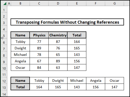
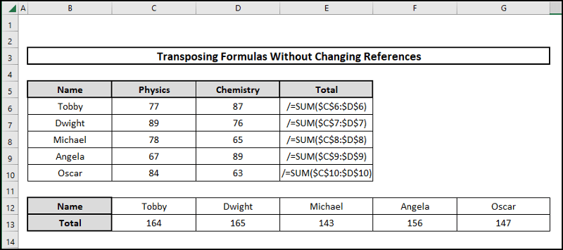
Let’s start by becoming familiar with our dataset, which we will use as an example throughout the article. In two rows, this spreadsheet contains the names of students, their test scores in Physics and Chemistry and the total marks in these two subjects. Now we want to convert the rows to columns, which means we want the name in the first column and their total marks in the second. Therefore, we will use this dataset to transpose formulas in the Total marks column in Excel without changing references.

This method will use Excel’s Paste Special feature to transpose formulas without changing references in Excel. When you paste copied cells into Excel, the copied text is automatically reformatted to match the destination content. You can, however, paste it as a link or an image or use Paste Special to keep the original formatting while transposing or swapping the rows and columns. Let us go through the steps to apply these functions.

⬇️⬇️ STEPS ⬇️⬇️

• Firstly, we have to add the cell references in the absolute form in the total marks column’s formula.

• Next, select the cells containing formulas you want to transpose without changing references. Here, we chose E6:E10 and copy the selected cells by pressing Ctrl+C simply.

• Now, select cell C13 and right-click on the cell, and select TRANSPOSE under the Paste option from the Context.

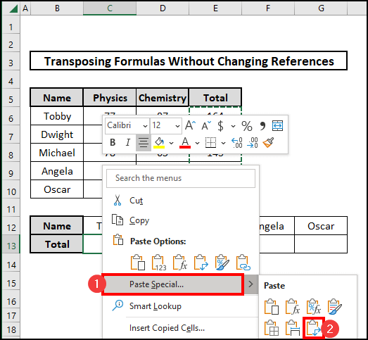
• Finally, we will have the name of the students and their total marks.

📕 Read More: Convert Column to Comma Separated List with Single Quotes

This second method will use the TRANSPOSE function option to transpose formulas without changing references in Excel. The TRANSPOSE function switches a horizontal range of cells into a vertical range or vice versa and must be entered as an array formula in a range with the same number of rows and columns as the source range. So, let us see the steps to apply this function.

⬇️⬇️ STEPS ⬇️⬇️

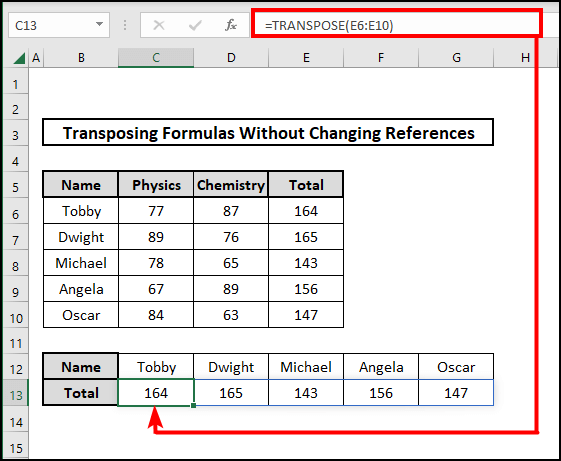
• Initially, choose the cell where you want to transpose the dataset first. We selected cell C13. Then, press Enter and the table will be transposed without formatting. Finally, you can customize the formatting of the table as you choose. We have formatted the table according to our format.

📕 Read More: Transpose Multiple Rows in Group to Columns with Formula in Excel

This method will use Find and Replace to transpose formulas without changing references. This feature of excel finds a certain text or character and replaces that with another text or character. Now, let us see the steps now.

⬇️⬇️ STEPS ⬇️⬇️

• Now, to transpose the Total marks column we will select E6:E10 and press Ctrl+H.

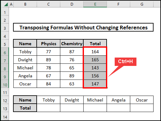
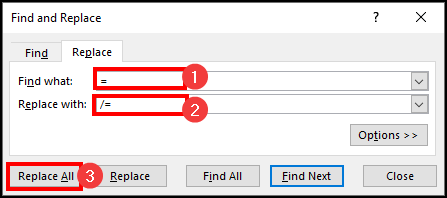
• Then, the Find and Replace named box will pop up. Type “=” in “Find What” and “/=” in the “Replace With” option and click on “Replace All”. The Total Marks column will get replaced with the defined character.

• Now, copy the range E6:E10, right-click on cell C13, and select TRANSPOSE under the Paste option from the Home tab in the Ribbon.

• After that, again select the cells C13:G13 and press Ctrl+H.

• Then, again type “/=” in the “Find What” and “=” in the “Replace With” option and click on “Replace All”.

• Finally, we will have our transposed dataset.

📕 Read More: 8 Ways to Transpose Multiple Rows in Group to Columns in Excel

This method will create a Pivot Table for transposing formulas without changing references in Excel. Let us see the steps now.

⬇️⬇️ STEPS ⬇️⬇️

• Initially, select the range B5:E10. Then, select Pivot Table from the Tables option of the Insert tab in the Ribbon.

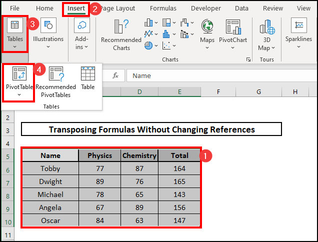
• Next, choose Existing Worksheet and insert B12 as the Location and press OK.

• After that, we will have PivotTable Fields on the right side of the sheet. Drag the Name and Total Marks field into the Columns.

• Lastly, we will have the outcome.

This method will apply Cell Reference directly to transpose formulas without changing references in Excel. This method will apply the cell reference directly where we want our results. Let us see the steps now.

⬇️⬇️ STEPS ⬇️⬇️

• First, insert the formula in cell C13.

• Now, we can do this manually if our dataset is not large. However, for a large dataset doing this manually can be tiresome. So, for the rest of the part, we will use Find and Replace.
• Now, to transpose the Total marks column we will select E6:E10 and press Ctrl+H.

• Then, the Find and Replace named box will pop up. Type “=” in “Find What” and “/=” in the “Replace With” option and click on “Replace All”. The Total Marks column will get replaced with the defined character.

• Now, copy the range E6:E10 and right-click on cell C13, and select TRANSPOSE under the Paste option from the Context.

• After that, again select the cells C13:G13 and press Ctrl+H.

• Then, again type “/=” in the “Find What” and “=” in the “Replace With” option and click on “Replace All”.

• Finally, we will have our transposed dataset.

📝 Takeaways from This Article

📌  This article demonstrated 5 methods to transpose formulas without changing references in Excel.

📌  In the first method, we employed Paste Special to transpose formulas without changing Excel references.

📌  Then, we demonstrated TRANSPOSE function to transpose formulas without changing references in Excel.

📌  After that, we applied Find and Replace feature for transposing formulas without changing references in Excel.

📌 Then, we employed Pivot Table to transpose formulas without changing references in Excel.

📌  Finally, we applied Cell References directly to transpose formulas without changing Excel references.

Conclusion

This article has demonstrated 5 methods to transpose formulas without changing references in Excel. All these formulas are incredibly effective and simple to use. We hope this article helps you. Please leave a remark if you have any queries. The author will do their best to find an appropriate answer.

For more guides like this, visit Excelden.com.