There may be times when you need to know how to extract data from Excel based on criteria. For example, you may need to use an Excel formula or VBA for this purpose. Today, we’ll show you to extract data based on criteria with various methods and lots of examples in Excel.
📁 Download Excel File
To prepare this article, we used an Excel workbook, which is available for download. Additionally, you can edit and customize the data you enter while viewing the results.
Learn to Extract Data from Excel Based on Criteria in 6 Different Ways
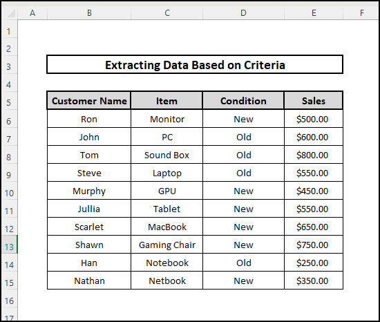
We may need to look for certain data to work with sometimes. But it’s very hard to find what we’re looking for when the dataset is very big. Here we are going to talk about 6 easy methods to extract data based on different criteria in Excel. We are going to extract data based on sales.
1. Array Formula to Get Data Based on Certain Criteria
Here we are going to extract data (sales amount) based on sales. We will use INDEX, IF, and MATCH functions. IF function enables you to compare a value to what you anticipate logically. Within a given table or range, the INDEX function will return either a value or a reference to a value. The MATCH function looks for a given item in a range of cells and returns the relative position of that item within the range. Also, the SMALL function returns the smallest value in a dataset. ROW function gives back the row number of a specific reference. Similarly COLUMN Function gives back the row number of a specific reference.
⬇️⬇️ STEPS ⬇️⬇️
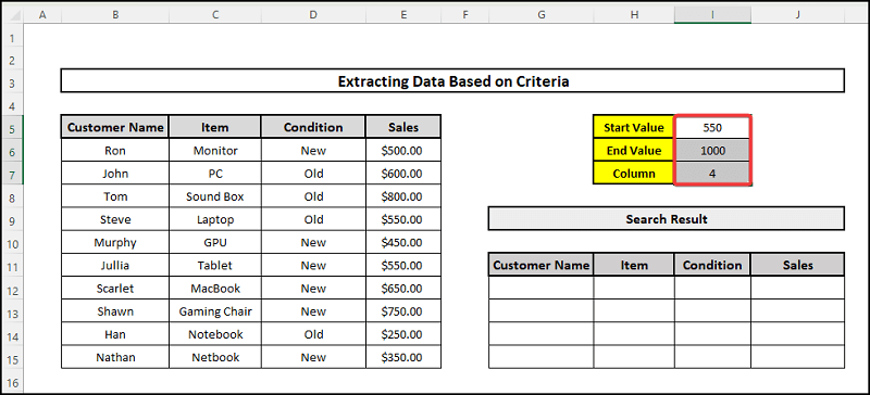
- At first, let’s put our criteria. We assume the start value of sales is $550 and the end value is $1000. The criteria range can be found in column 4. So we put these values in cells I5, I6, and I7.
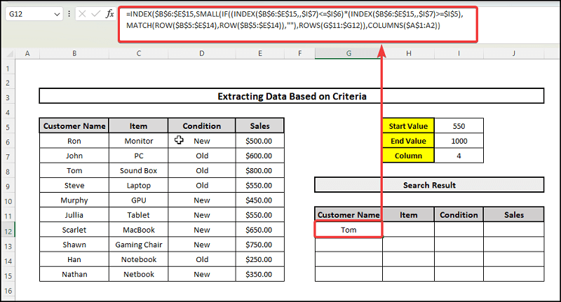
- Then we select cell G12. Then we put the formula below:
MATCH(ROW($B$6:$E$15),ROW($B$6:$E$15)),””) returns one specific value if logical test here is TRUE and FALSE otherwise.
🔨 Formula Breakdown👉 (INDEX($B$6:$E$15,,$I$7)<=$I$6)*(INDEX($B$6:$E$15,,$I$7)>=$I$5) indicates that the numbers 1 and 0 represent TRUE and FALSE, respectively (zero). When the arithmetic operation is done in a formula, they are changed.👉 ROW($B$6:$E$15) calculates the number of rows of the reference.👉 MATCH(ROW($B$6:$E$15),ROW($B$6:$E$15)) returns relative position of the item.👉 IF((INDEX($B$6:$E$15,,$I$7)<=$I$6)*(INDEX($B$6:$E$15,,$I$7)>=$I$5),👉 SMALL(IF((INDEX($B$6:$E$15,,$I$7)<=$I$6)*(INDEX($B$6:$E$15,,$I$7)>=$I$5),MATCH(ROW($B$6:$E$15),ROW($B$6:$E$15)),””),ROWS(G12:$G$12)) returns the smallest value.
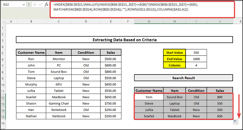
- Then we press Enter and drag down the formula to cell The final result will be like this.
📕 Read More: Extract Data from Table Based on Multiple Criteria in Excel
2. Using Array formula for More Than One Condition
Here we are going to extract data based on sales. We will use INDEX, IF, COUNTIF, and MATCH functions. IF function enables you to compare a value to what you anticipate logically. This formula uses the COUNTIF function to find each name of one Column in another Column. For each piece of data in the first Column, the function will give back a number that shows how many times it found a match. Within a given table or range, the INDEX function will return either a value or a reference to a value. The MATCH function looks for a given item in range of cells and returns the relative position of that item within the range. Also, the SMALL function returns the smallest value in a dataset. ROW function gives back the row number of a specific reference. Similarly, COLUMN Function gives back the row number of a specific reference
⬇️⬇️ STEPS ⬇️⬇️
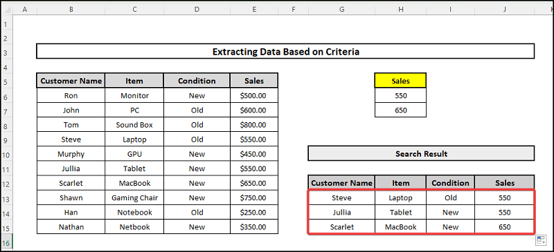
- At first, let’s put our criteria. We assume the start value of sales is $550 and the end value is $650. So we put these values in cells H6 and H7.

- Then we select cell G13. Then we put the formula below:

MATCH(ROW($B$6:$E$15),ROW($B$6:$E$15)),””) returns one specific value if the logical test is TRUE and a different value if the logical test is FALSE.
🔨 Formula Breakdown👉 IF(COUNTIF($H$7:$H$7,$E$6:$E$15), MATCH(ROW($B$6:$E$15), ROW($B$6:$E$15)), “”) Here it takes three arguments. Within them, the first of which has to be a logical declaration. If this expression is TRUE, the output is the second argument, and in the case of FALSE, the output is another (argument 3). Step 1 determined this logical expression: TRUE = 1, FALSE = 0. (zero).👉 (INDEX($B$6:$E$15,,$I$7)<=$I$6)*(INDEX($B$6:$E$15,,$I$7)>=$I$5) indicates that the numbers 1 and 0 represent TRUE and FALSE, respectively (zero). When an arithmetic operation is done in a formula, they are changed.👉 ROW($B$6:$E$15) calculates the number of rows of the reference.👉 MATCH(ROW($B$6:$E$15),ROW($B$6:$E$15)) returns the relative position of an item.👉 IF((INDEX($B$6:$E$15,,$I$7)<=$I$6)*(INDEX($B$6:$E$15,,$I$7)>=$I$5),👉 SMALL(IF((INDEX($B$6:$E$15,,$I$7)<=$I$6)*(INDEX($B$6:$E$15,,$I$7)>=$I$5),MATCH(ROW($B$6:$E$15),ROW($B$6:$E$15)),””),ROWS(G12:$G$12)) returns the smallest value.
- Then we press Enter and drag down the formula to cell.
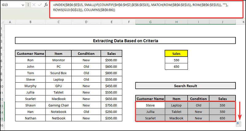
- The final result will be like this.
📕 Read More: Pull Same Cell from Multiple Sheets into Master Column
3. Utilizing Filter Feature
Filter Command Feature is a powerful tool for calculating, summarizing, and analyzing data that lets you see comparisons, various patterns, and some trends in the data. Now I’ll demonstrate how to count the number of occurrences that occur each day by using Filter Command Tool.
⬇️⬇️ STEPS ⬇️⬇️
- Firstly, we select the headers of our dataset.
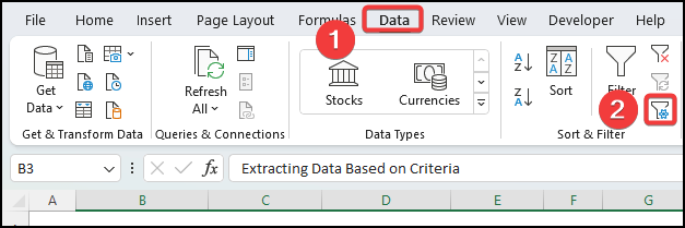
- Then we select Data tab and select Filter.
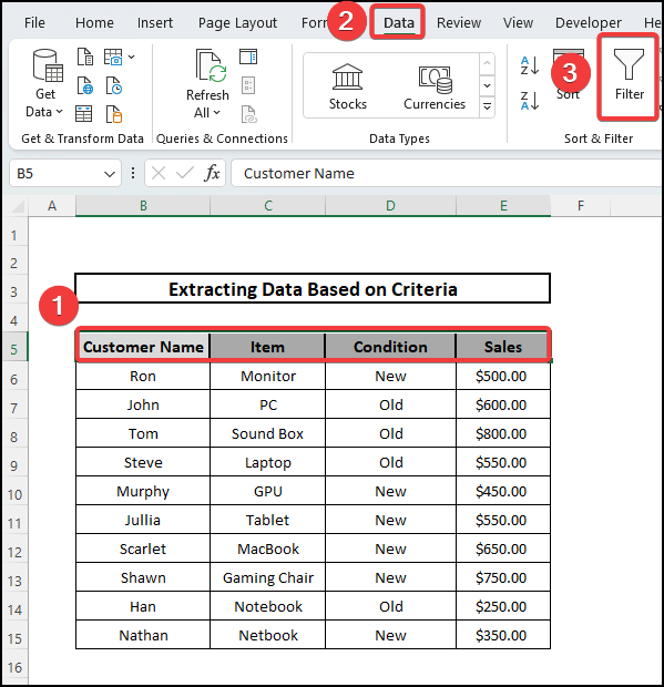
- The result will be like this.
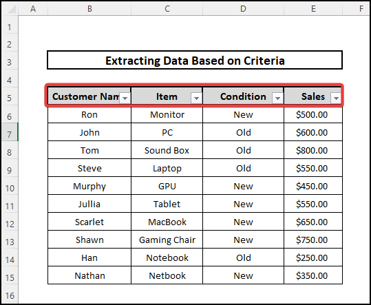
- Now we go to the Sales header and from drop-down box and then Number Filters and then Between…
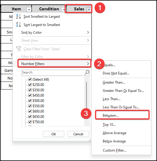
- Now, in the next pop-up Custom AutoFilter section, we select 550 from drop-down list that appears when we click on drop-down button that is next to the is greater than or equal to header, and we also choose 600 in the header box that says is less than or equal to. Then we press Ok.

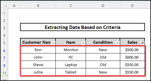
- Here is our result.
4. Implementing Advanced Filter
Advance Filter Command Tool is a powerful tool for calculating, summarizing, and analyzing data that lets you see comparisons, various patterns, and some trends in the data. Now I’ll demonstrate how to count the number of occurrences that occur each day by using the Advance Filter Command Tool.
⬇️⬇️ STEPS ⬇️⬇️
- First, we select the entire dataset.
- Then we select Data tab and select Advanced.
- After that, range of our chosen data will be shown in a box next to List range
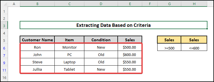
- Then in a box next to Criteria range, we choose the cells that have the conditions you set. After cell reference numbers that hold predefined conditions, the name of the worksheet will be filled in automatically.
- Now click OK to finish.

- Here is our result.
5. Getting Data from Table
Using Filter option on an Excel worksheet, you can get data from an Excel table. The steps are as below.
⬇️⬇️ STEPS ⬇️⬇️
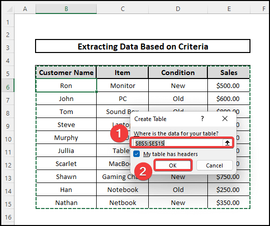
- Choosing a cell from the dataset, we press Ctrl and T.
- In the new box “Create Table”, we put the range. Then press OK in the box.
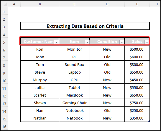
- It will look like this.
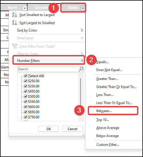
- Now we go to the Sales header and from drop-down box and choose Number Filters and then Between…
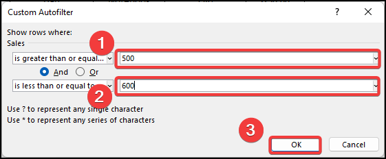
- Now, in the next pop-up Custom AutoFilter box, we select 550 from drop-down list that appears when we click on drop-down button that is next to the is greater than or equal to header, and we also choose 600 in the header box that says is less than or equal to. Then we press OK.
- Here is our result.
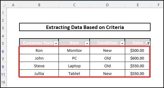
6. Extracting Data to Another Worksheet
We can extract data from another worksheet. The process is almost the same as using an Advance Filter.
⬇️⬇️ STEPS ⬇️⬇️
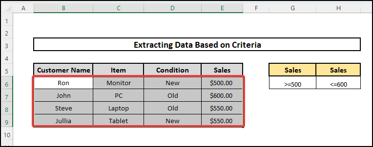
- First, we define criteria as we are looking for sales between $500 and $600.
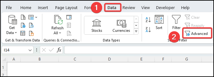
- Then in the new worksheet, we select Data tab and select Advanced.
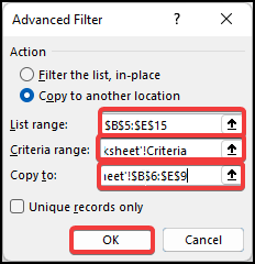
- After that, we select Copy to another location. Then we put range of our chosen data will be shown in a box next to List range box.
- Then, in a box next to Criteria range, we choose the cells that have the conditions you set. After cell reference numbers that hold predefined conditions, the name of the worksheet will be filled in automatically.
- We put the location of the result next to the Copy to box.
- Now click OK to finish.
- Here is our result.
📕 Read More: 5 Ways to Extract Filtered Data into Another Excel Sheet
How to Extract Specific Number from Cell in Excel
Here we can also extract a specific number from a cell in Excel. We will use several functions here. We will use the INDEX function that will return either a value or a reference to a value. To count the matches alongside two columns, we can only use the SUMPRODUCT function. The SUMPRODUCT function counts and adds up all the ones and zeros in an array. The ISNUMBER function checks to see if the data in a cell is a number (TRUE) or not (False). ROW function gives back the row number of a specific reference. Similarly, the COLUMN Function gives back the row number of a specific reference
For that we can follow the below steps:
⬇️⬇️ STEPS ⬇️⬇️
- At first, we select cell C6. Then we put the formula below:
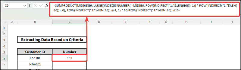
🔨 Formula Breakdown👉 (INDIRECT(“1:”&LEN(B6))), 0) it searches by the length of the text put in cell B6.👉 ROW(INDIRECT(“1:”&LEN(B6))), 0 calculates the number of rows of the reference.👉 (ISNUMBER(–MID(B6, ROW(INDIRECT(“1:”&LEN(B6))), 1)) returns the largest value returned by the INDIRECT function. ISNUMBER converts the array that came by the MID function to TRUE or FALSE.👉 LARGE(INDEX(ISNUMBER(–MID(B6, ROW(INDIRECT(“1:”&LEN(B6))),1)) Here LARGE Function returns the largest value returned by the INDEX function that will return either a value or a reference to a value.👉 SUMPRODUCT returns the whole row here.
- Then we press Enter and drag down the formula.
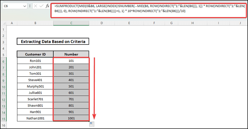
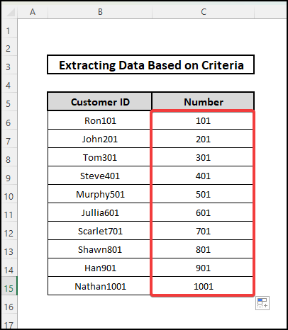
- The final result will be like this.
📕 Read More: 4 Ways to Pull Values in Excel from Another Worksheet
📄 Important Notes
🖊️ In Excel, the ribbon is used to access various commands. You can change a lot of things in the options dialogue window, like the ribbon, formulas, proofing, saving, and so on. So the appearance of worksheets on your device could be different from ours.
🖊️ A practice workbook is given so that you can practice yourself.
🖊️ All these exercises and tutorials are done on Microsoft Office 365. Some functions may be unavailable in previous versions.
🖊️ At the side of each Excel worksheet file, there is space where they can practice.
📝 Takeaways from This Article
📌 Readers will be able to know easily how to extract data from excel on criteria with various methods.
📌 They can utilize the Array formula.
📌 They can also use the Array formula with multiple conditions.
📌 Readers can also implement Excel Filter Command.
📌 The readers can again extract data from a different worksheet.
📌 Readers can again extract data from Excel defined table.
Conclusion
That concludes today’s session. These are the methods for using Excel to extract data from excel based on criteria. Hopefully, it was helpful to you. Don’t forget to leave your thoughts and questions in the comments section and explore our website, ExcelDen.com, the best Excel solutions provider.


