The VLOOKUP function is basically used to search values vertically, and it’s a very easy and useful tool in Excel. This article will discuss how to utilize the Excel VLOOKUP formula with multiple sheets. This function actually returns dates, strings, numerical values, etc.
📁 Download Excel File
Download the Excel file we used to create this article so you can practice.
Learn to Utilize VLOOKUP Function with Multiple Sheets Using Excel Formula with These 5 Examples
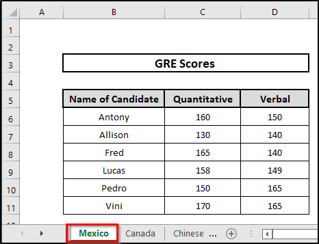
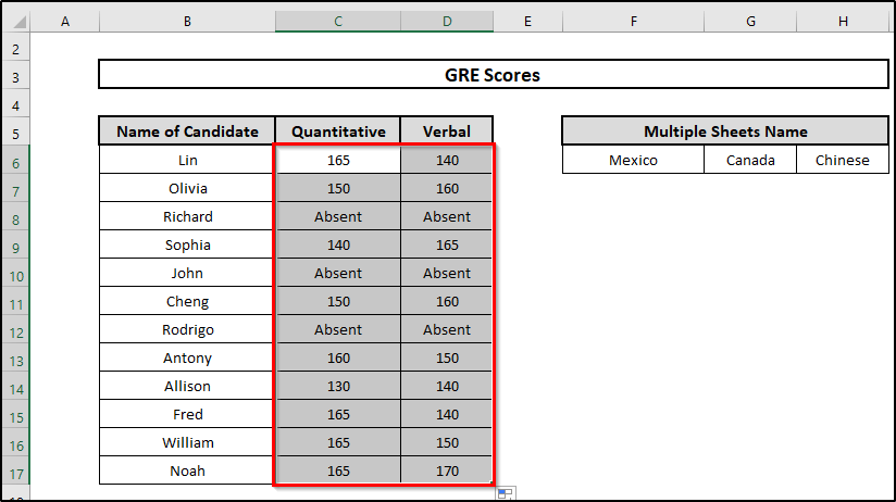
There are several ways of using the VLOOKUP formula with several sheets. We used three datasets that contained GRE scores from admission candidates from three different countries.
In our first sheet, scores of candidates from Mexico are given.
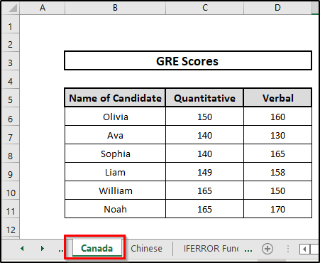
The scores of Canadian candidates are shown on the following sheet.
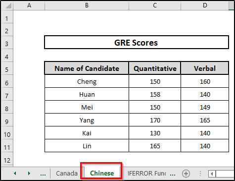
On the third sheet, scores for Chinese candidates are given.
1. Integrating Multiple Functions
You can combine multiple functions with VLOOKUP to achieve your goal. The functions that you can use with VLOOKUP are IFERROR, INDIRECT, MATCH, and COUNTIF functions.
Let’s see how to do this with some simple steps.
⬇️⬇️ STEPS ⬇️⬇️
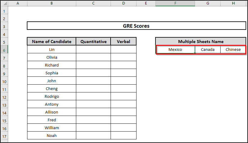
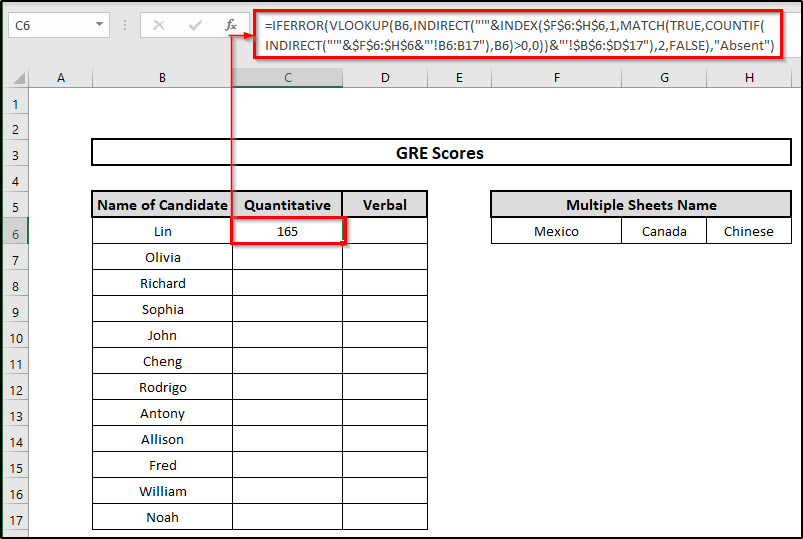
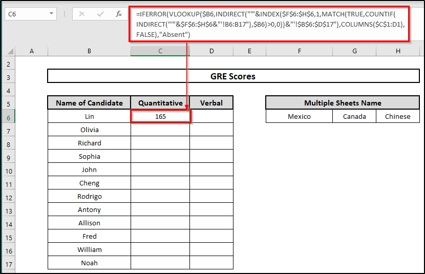
- First, in any part of your worksheet, name the other sheets you’ll be looking at for data. Here, we have created an array with other sheets’ names on cell F6:H6.
- After that, insert the given formula, we have inserted the formula given below in cell C6.
=IFERROR(VLOOKUP(B6,INDIRECT(“‘”&INDEX($F$6:$H$6,1,MATCH(TRUE,COUNTIF(INDIRECT(“‘”&$F$6:$H$6&”‘!B6:B17″),B6)>0,0))&”‘!$B$6:$D$17″),2,FALSE),”Absent”)
🔨 Formula Breakdown
IFERROR(VLOOKUP(B6,INDIRECT(“‘”&INDEX($F$6:$H$6,1,MATCH(TRUE,COUNTIF(INDIRECT(“‘”&$F$6:$H$6&”‘!B6:B17″),B6)>0,0))&”‘!$B$6:$D$17″),2,FALSE),”Absent”)
👉 The number of times the value in cell B6 is present in the range Mexico is first provided by COUNTIF(INDIRECT(“‘”&$F$6:$H$6&”‘!B6:B17”)! Canada, B6:B17 Chinese, and B6:B17! B6–B17, in that order.
👉 The worksheet names are $F$6:$H$6 in this instance. As a result, “Sheet Name” is passed to the INDIRECT formula! B6:B17. The function’s return value in this section is, therefore {0, 0, 1}.
👉 This causes MATCH(TRUE,COUNTIF(INDIRECT(“‘”&$F$6:$H$6&”‘!B6:B17”),$B6)>0,0) to change into MATCH(TRUE,0,0,1>0,0), which returns the worksheet that has the value in B6. In this case, the result is 3.
👉 As the value in B6 (Lin) is found in worksheet no. 3, it thus returned 3 ( Chinese).
👉 This causes INDEX($F$6:$H$6,1,MATCH(TRUE,COUNTIF(INDIRECT(“‘”&$F$6:$H$6&”‘!B6:B17”),$B6)>0,0) to change into INDEX($F$6:$H$6,1,3), which is in charge of returning the precise name of the worksheet where the value in cell B6 is. Therefore, it gives value Chinese.
👉 Therefore, the INDIRECT function becomes, INDIRECT(“‘”&Chinese&”‘!$B$6:$D$11”) and provides the total cell ranges in which the value in B6 is present. As a result, the output becomes,{“Cheng”,150,160;”“Huan”,158,140;”“Mei”,150,149;”“Yang,170,165;”“Kai ,130,140;”“Lin,165,140”}.
👉 Last but not least, VLOOKUP($B6,”Cheng”,150,160;”Huan”,158,140;”Mei”,150,149;”Yang,170,165;”Kai,130,140;”Lin,165,140″,2,FALSE) returns the second column of the row from that range where the value in cell B6 matches. The result is 165, which is the score we wanted on the quantitative exam.
👉 Because we nested the name within an IFERROR function, it will return “Absent” if the name cannot be found in any worksheet.
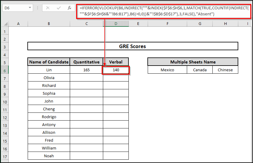
- After that, on the other cell enter the formula below.
=IFERROR(VLOOKUP(B6,INDIRECT(“‘”&INDEX($F$6:$H$6,1,MATCH(TRUE,COUNTIF(INDIRECT(“‘”&$F$6:$H$6&”‘!B6:B17″),B6)>0,0))&”‘!$B$6:$D$17″),3,FALSE),”Absent”)
- Next, we have to fill the available cells. Use Fill Handle and drag it toward the end. You will see that the cells are now filled.
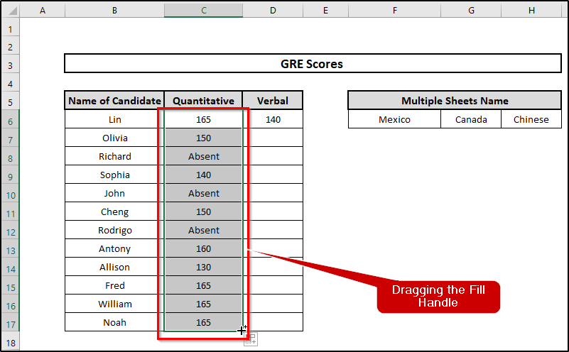
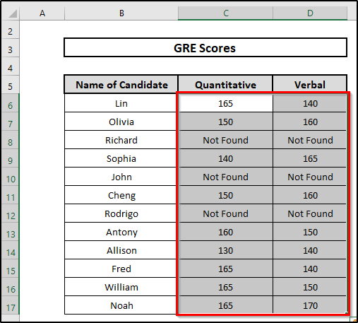
- Notice that data the missing data from those three cells are shown as Absent in that sheet, and the rest of the sheet is filled with data torn from those three sheets.
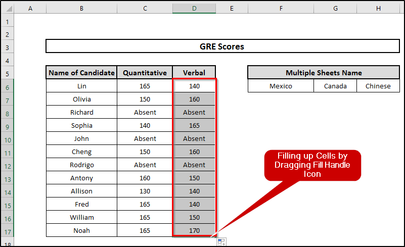
- Finally, follow the same process of dragging the icon of Fill Handle for the adjacent cell to fill up.
📕 Read More: VLOOKUP to Find Duplicates in Two Columns in Excel
2. Combining IFERROR and VLOOKUP Functions
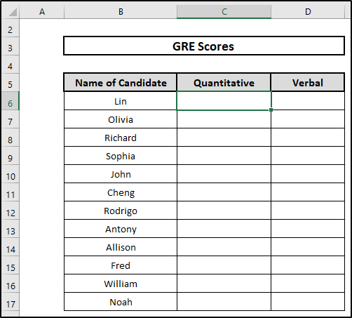
We can combine VLOOKUP with the IFERROR function. This function searches data in multiple worksheets one by one. Suppose this is a worksheet that contains the names of all candidates. Now, we want to find out who among these people has submitted their GRE scores. Let’s follow the steps below.
⬇️⬇️ STEPS ⬇️⬇️
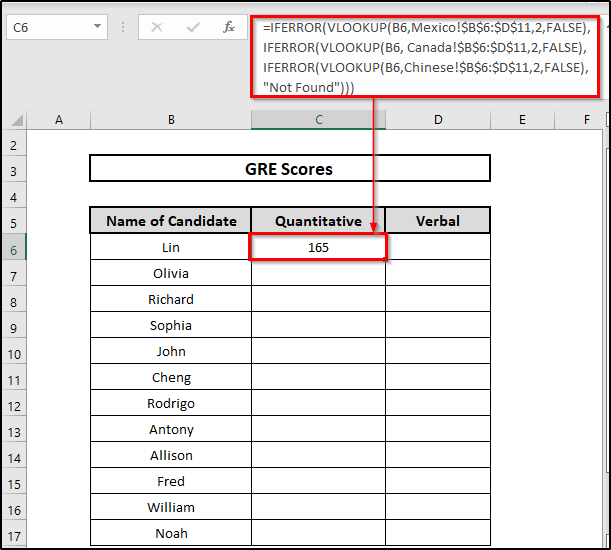
- First, we’ll look up the results from the first worksheet. To do this, we have entered the formula given below in the cell of the quantitative score, which is C6. Enter the formula and see the data.
The formula is given below.
=IFERROR(VLOOKUP(B6,Mexico!$B$6:$D$11,2,FALSE),IFERROR(VLOOKUP(B6, Canada!$B$6:$D$11,2,FALSE),IFERROR(VLOOKUP(B6,Chinese!$B$6:$D$11,2,FALSE),”Not Found”)))
🔨 Formula Breakdown
IFERROR(VLOOKUP(B6,Mexico!$B$6:$D$11,2,FALSE),IFERROR(VLOOKUP(B6, Canada!$B$6:$D$11,2,FALSE),IFERROR(VLOOKUP(B6,Chinese!$B$6:$D$11,2,FALSE),”Not Found”)))
Let’s analyze the nested IFERROR function by its syntax.
👉 B6 is the lookup_value, Mexico refers sheet 1 and $B$6:$D$11 is the table_array of that sheet. The col_index_number is represented by 2.So,VLOOKUP(B6,Mexico!$B$6:$D$11,2,FALSE) is to look up the value in sheet 1.
👉 Then comes the IFERROR function, which says that if the value is not found in the first referred sheet then lookup this value in the other two sheets, which is represented by following the same syntax. VLOOKUP(B6, Canada!$B$6:$D$11,2,FALSE) searches in the 2nd sheet, and if this returns False, which means the value is not in that sheet it goes to look in sheet 3 by VLOOKUP(B6,Chinese!$B$6:$D$11,2,FALSE).
👉 And finally, if this value is not even found in the last sheet it will show up the message “Not Found”.
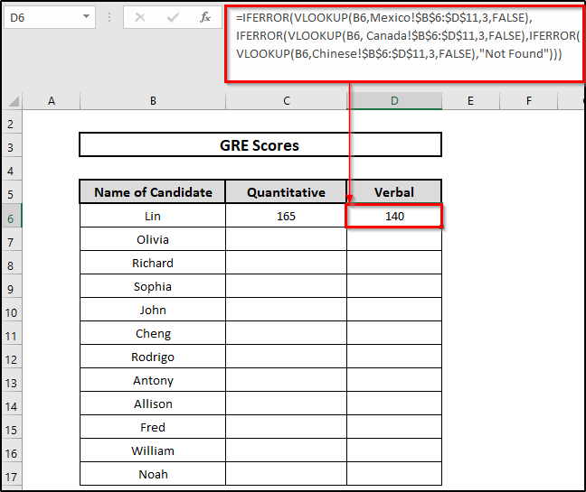
- After that, for the next cell, you have to apply almost the same formula but with modifications. Here is the formula that we have used.
=IFERROR(VLOOKUP(B6,Mexico!$B$6:$D$11,3,FALSE),IFERROR(VLOOKUP(B6, Canada!$B$6:$D$11,3,FALSE),IFERROR(VLOOKUP(B6,Chinese!$B$6:$D$11,3,FALSE),”Not Found”)))
- After that, select all cells and use the icon of Fill Handle to fill up the remaining cells.
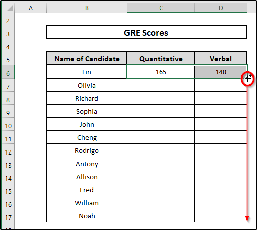
- Finally, after dragging Fill Handle icon downward, you will find the cells are filled, and the data that was not on those three sheets have shown the message Not Found.
📕 Read More: 8 Ways to VLOOKUP to Return Multiple Values Vertically in Excel
3. Utilizing Dynamic Column Index Number
In other approaches of Excel VLOOKUP in multiple sheets formula, formulas are inserted in every cell. In other processes, col_index_num is defined as 2 to extract the quantitative marks and 3 to obtain the verbal marks. But in this example, we are going to use COLUMNS($C$1:D1) instead of col_index_num . Follow the steps illustrated below to learn more.
⬇️⬇️ STEPS ⬇️⬇️
- Firstly, insert the sheets name in any cells on your worksheet. We have used the cell range F6:H6.
- After that, Enter the given formula.
=IFERROR(VLOOKUP($B6,INDIRECT(“‘”&INDEX($F$6:$H$6,1,MATCH(TRUE,COUNTIF(INDIRECT(“‘”&$F$6:$H$6&”‘!B6:B17″),$B6)>0,0))&”‘!$B$6:$D$17″),COLUMNS($C$1:D1),FALSE),”Absent”)
🔨 Formula Breakdown
IFERROR(VLOOKUP($B6,INDIRECT(“‘”&INDEX($F$6:$H$6,1,MATCH(TRUE,COUNTIF(INDIRECT(“‘”&$F$6:$H$6&”‘!B6:B17″),$B6)>0,0))&”‘!$B$6:$D$17″),COLUMNS($C$1:D1),FALSE),”Absent”)
👉 Firstly, the function COUNTIF(INDIRECT(“‘”&$F$6:$H$6&”‘!B6:B17”) shows how many occasions the cell $B6 has occurred in the required range Mexico!B6:B17, Canada!B6:B17 and Chinese!B6:B17 respectively.
👉 Here $F$6:$H$6 is worksheet’s name. Therefore, INDIRECT formula takes ‘Sheet_Name’!B6:B17.So this part of the function returns the value {0,0,1}.
👉 Then , MATCH(TRUE,COUNTIF(INDIRECT(“‘”&$F$6:$H$6&”‘!B6:B17”),$B6)>0,0) becomes MATCH(TRUE,{0,0,1}>0,0), which provides the worksheet value in B6 is present.Here, the output becomes 3.
👉 It provided 3 because the amount in B6 (Lin) is in 3rd worksheet ( Chinese).
👉 After that,INDEX($F$6:$H$6,1,MATCH(TRUE,COUNTIF(INDIRECT(“‘”&$F$6:$H$6&”‘!B6:B17”),$B6)>0,0) becomes INDEX($F$6:$H$6,1,3)which is responsible for returning the worksheet’s name where the cell B6 is located. So, it returns the value Chinese.
👉 Then, the INDIRECT function becomes, INDIRECT(“‘”&Chinese&”‘!$B$6:$D$11”) and returns the all cells range. As a result, the output becomes,{“Cheng”,150,160;”“Huan”,158,140;”“Mei”,150,149;”“Yang,170,165;”“Kai ,130,140;”“Lin,165,140”}.
👉 Also, the function COLUMNS($C$1:D1) refers to the column number, which we are searching for. Here it returns 2.
👉 And so, VLOOKUP($B6,{“Cheng”,150,160;”“Huan”,158,140;”“Mei”,150,149;”“Yang,170,165;”“Kai ,130,140;”“Lin,165,140”},2,FALSE) provides the range’s second column and row, where cell B6’s value is the match. The output becomes 165. So, it is the required quantitative exam mark.
👉 On the other hand if The name cannot be available in another worksheet, that will provide “Absent”.
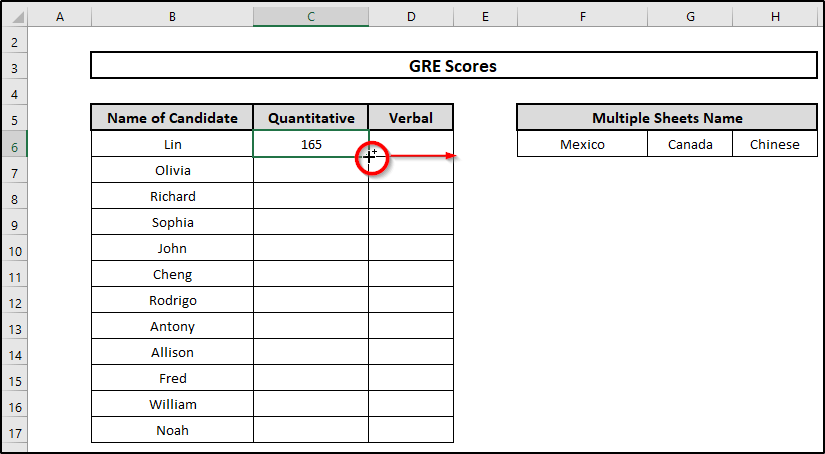
- Now, you can drag Fill Handle icon and fill it up. We obtained the verbal marks by dragging Fill Handle icon from the side of the quantitative marks.
- Finally, drag the Fill Handle icon again downwards to fill up the other cells below.
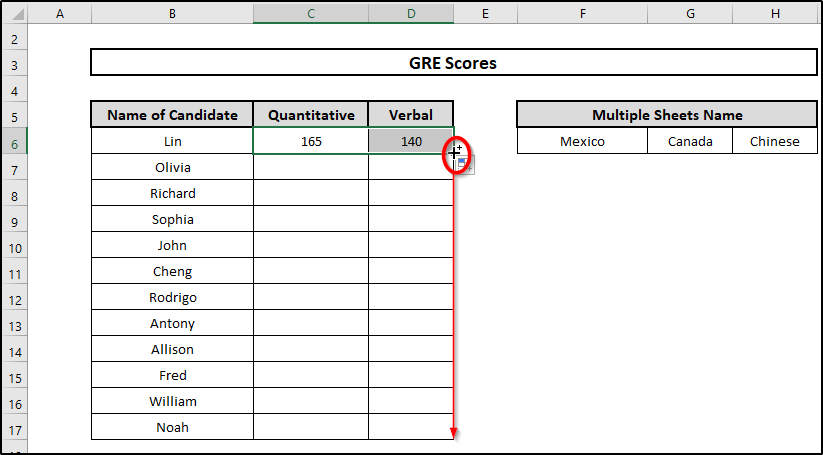
- So, you have filled up all the cells by just inserting the formula into one of the cells.
📕 Read More: 5 Ways to Extract Filtered Data into Another Excel Sheet
4. Applying INDIRECT Function
To use Excel VLOOKUP in multiple sheets formula you can also integrate it with the INDIRECT function. To know how to do this, follow the steps below.
- First, in any of the cells in your worksheet, write the sheets name that you would like to search for. We have selected an array in cell F6:H6.
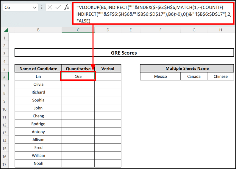
- Then Enter the given formula in your preferred cell; we have used cell C6.
=VLOOKUP(B6,INDIRECT(“‘”&INDEX($F$6:$H$6,MATCH(1,–(COUNTIF(INDIRECT(“‘”&$F$6:$H$6&”‘!$B$6:$D$17″),B6)>0),0))&”‘!$B$6:$D$17”),2,FALSE)
🔨 Formula Breakdown
VLOOKUP(B6,INDIRECT(“‘”&INDEX($F$6:$H$6,MATCH(1,–(COUNTIF(INDIRECT(“‘”&$F$6:$H$6&”‘!$B$6:$D$17″),B6)>0),0))&”‘!$B$6:$D$17”),2,FALSE)
👉 At first, COUNTIF(INDIRECT(“‘”&$F$6:$H$6&”‘!B6:B17”) provides how many occasions the cell B6 is available in range Mexico!B6:B17, Canada!B6:B17 and Chinese!B6:B17 respectively.
👉 Here $F$6:$H$6 is the worksheet’s name. Therefore, INDIRECT formula takes ‘Sheet_Name’!B6:B17.So this part of the function returns the value {0,0,1}.
👉 Then , MATCH(1,–,COUNTIF(INDIRECT(“‘”&$F$6:$H$6&”‘!B6:B17”),$B6)>0,0) becomes MATCH(TRUE,{0,0,1}>0,0), which provides the worksheet value in B6 is present.Here, the output becomes 3.
👉 It gives 3 because cell value in B6 (Lin) lies in worksheet no 3 ( Chinese).
👉 After that,INDEX($F$6:$H$6,1,MATCH(TRUE,COUNTIF(INDIRECT(“‘”&$F$6:$H$6&”‘!B6:B17”),$B6)>0,0) becomes INDEX($F$6:$H$6,1,3)which is responsible for giving the worksheet name where the cell value B6 is. So, it returns the value Chinese.
👉 Then, the INDIRECT function becomes, INDIRECT(“‘”&Chinese&”‘!$B$6:$D$11”) and provides the overall range of cells in which value in B6 is present. Therefore, the output becomes,{“Cheng”,150,160;”“Huan”,158,140;”“Mei”,150,149;”“Yang,170,165;”“Kai ,130,140;”“Lin,165,140”}.
👉 And so, VLOOKUP($B6,{“Cheng”,150,160;”“Huan”,158,140;”“Mei”,150,149;”“Yang,170,165;”“Kai ,130,140;”“Lin,165,140”},2,FALSE) delivers the row from that range’s second column where the value in cell B6 matches. The output becomes 165. So, This is the score on the quantitative exam that we were after..
👉 On the other side, it will display N/A or an error if the name is not present in any worksheet.
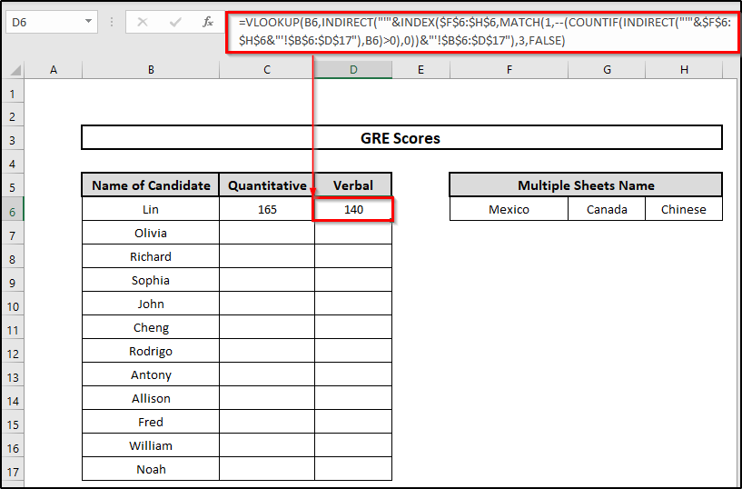
- After that, use the formula below to fill up the adjacent cell. This formula is quite the same as the previous one, but with a bit more cell modification.
=VLOOKUP(B6,INDIRECT(“‘”&INDEX($F$6:$H$6,MATCH(1,–(COUNTIF(INDIRECT(“‘”&$F$6:$H$6&”‘!$B$6:$D$17″),B6)>0),0))&”‘!$B$6:$D$17”),3,FALSE)
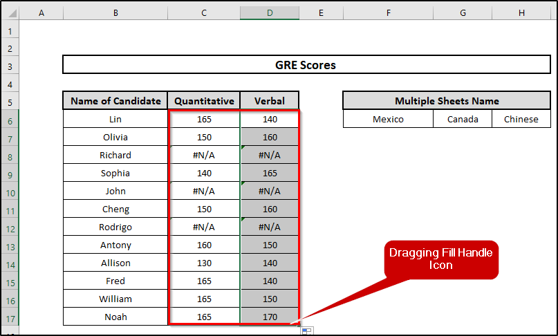
- In the next step, you have to use Fill Handle in order to fill up the rest of the cells in that column. Drag the icon of Fill Handle downward, and you will find that you have filled the rest of the cells.
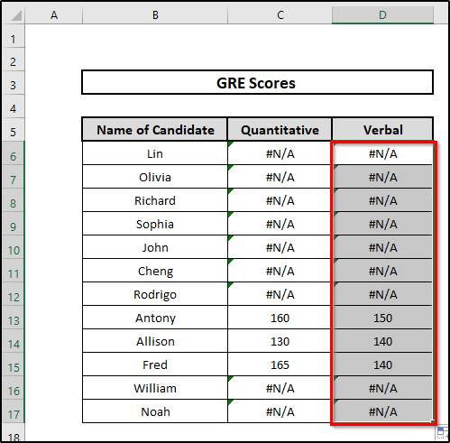
- Follow the same steps for the adjacent column, using Fill Handle icon in order to fill it up. Notice that the data that was not available in those three sheets is now showing the message error or N/A in both of the columns.
📕 Read More: 6 Solutions If VLOOKUP Returns #N/A When Match Exists in Excel
5. Exploring Across Each Worksheet Separately Utilizing VLOOKUP Only
We can also use the Excel VLOOKUP in multiple sheets formula only to search the data in multiple worksheets at the same time. However, keep in mind that by using this function, we will be able to search within each individual worksheet. See the following steps below to know more.
⬇️⬇️ STEPS ⬇️⬇️
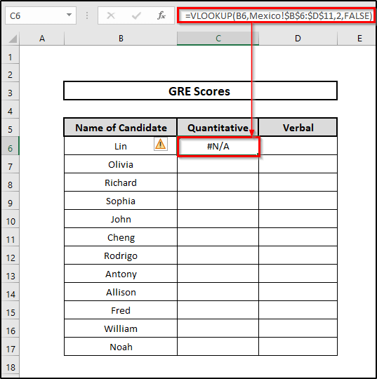
- First, select the cell where you would like to see the extracted value. We have chosen cell C6.
- Now Enter the given formula in your preferred cell.
=VLOOKUP(B6,Mexico!$B$6:$D$11,2,FALSE)
🔨 Formula Breakdown
VLOOKUP(B6,Mexico!$B$6:$D$11,2,FALSE)
Here,
👉 B6 is the lookup_value, which indicates the cell number, where we have stored the value that we are looking for in other sheets.
👉 Mexico is the sheet name where we are searching for that value. As we are searching it in individual sheets separately, we have to change this to search in other sheets.
👉 $B$6:$D$11 is the table_array, to specify the table in that sheet where to search for data.
👉 2 is the col_index_number.
👉 False is the [range_lookup]
👉 This means the function takes an argument which is a range of cells, by table_array,then searches for specific value by lookup_value argument in the initial column of the array.
👉 It looks for an exact match by the [range_lookup], False and if it is not available in that sheet, it shows a N/A or error, here as the result of Lin was not available in the first sheet, it is showing the error.
👉 But if it finds the exact match of lookup_value in the first column of the table_array, it moves a few steps right for a specific column col_index_number and returns the value of this column.
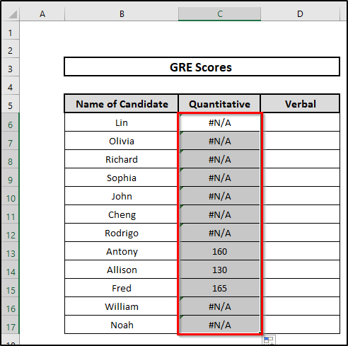
- After that, you need to use Fill Handle icon again in order to fill up the other cells.

- And notice that, the values which were available only in the first sheet have been shown; otherwise, it’s displaying an error.
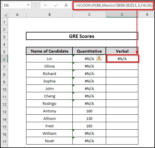
- After completing one column, just follow the same process for the next column. Enter the given formula.
=VLOOKUP(B6,Mexico!$B$6:$D$11,3,FALSE)
- Utilize Fill Handle icon just as before to fill all the cells in that column.
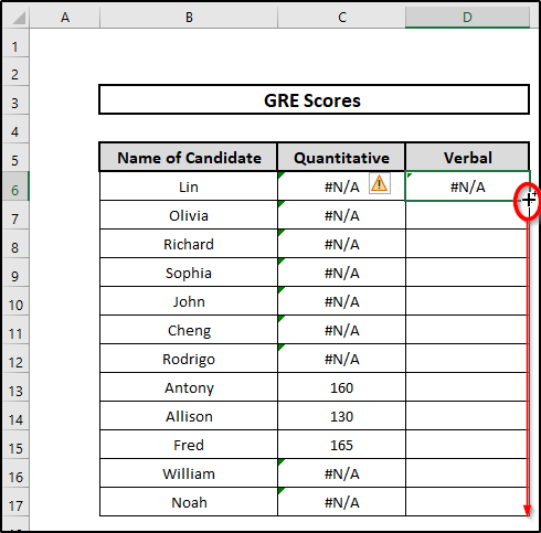
- By dragging the icon of Fill Handle downward, we have filled the entire column.
Furthermore, you can follow this process and search all the other sheets available. The main disadvantage of this process is that you have to enter functions individually for all sheets, which will be a tedious process if you have many worksheets to search for.
However, this process is a useful one because the formula is quite simple in comparison to other formulas.
📕 Read More: What Is Table Array in VLOOKUP in Excel?
📝 Takeaways from This Article
📌 You can now search multiple sheets individually or together.
📌 After reading this article you can now use the combinations of formulas that you have learned and used effectively.
Conclusion
VLOOKUP is a blessing for Excel users, as it saves lots of time and effort for them, making it very easy to use. So, we will recommend that you use any of the formulas mentioned above whenever you have to take data from spreadsheets. We have shown five effective examples to use the VLOOKUP function with multiple sheets using the Excel formula. Please leave a comment if you want to give any suggestions or questions. Don’t forget to visit our Excelden page to enhance your Excel-related knowledge.
Related Articles
- 7 Ways to Use VLOOKUP to Compare Two Lists
- Find MAX of Multiple Values Using VLOOKUP Function in Excel
- 5 Examples to Use IF and VLOOKUP as Nested Function in Excel
- 2 Ways to Use VLOOKUP Function with Two Lookup Values
- 3 Quick Ways to Vlookup and Return Multiple Values Horizontally


