In this lesson, I’ll demonstrate 8 effective approaches on how to Use VLOOKUP to return multiple values vertically in Excel. Finally these techniques will enable you to solve the problem that led you here. You will master several crucial Excel features and functions during this article, which will come in extremely handy for any assignment using Excel.
📁 Download Excel File
The sample worksheet that was used during the discussion is available to download for free right here.
Learn to Use VLOOKUP to Return Multiple Values Vertically in Excel with These 8 Methods
Here we have a dataset of different Movies’ list with their corresponding Movie type, Directors and IMDB Ratings. Therefore, we are going to use bunch of different methods using different functions to filter out data.
1. Vlookup Using FILTER Function
Here we will be using the FILTER function to VLOOKUP and return multiple values vertically
⬇️⬇️ STEPS ⬇️⬇️
- Firstly copy down the following formula in a cell to VLOOKUP.
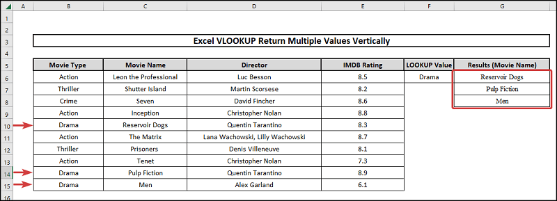
=FILTER(C6:C15, F6=B6:B15)
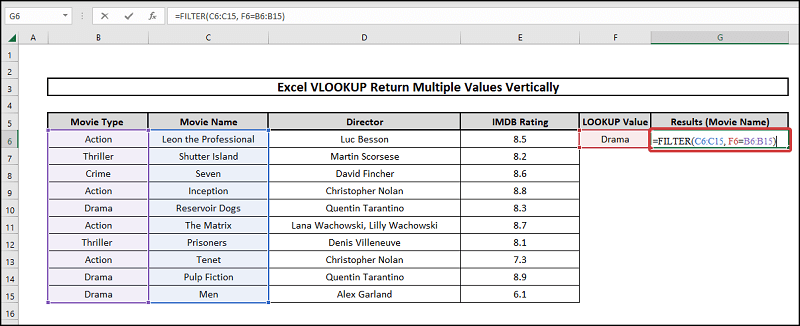
- After that press Enter to get the results.
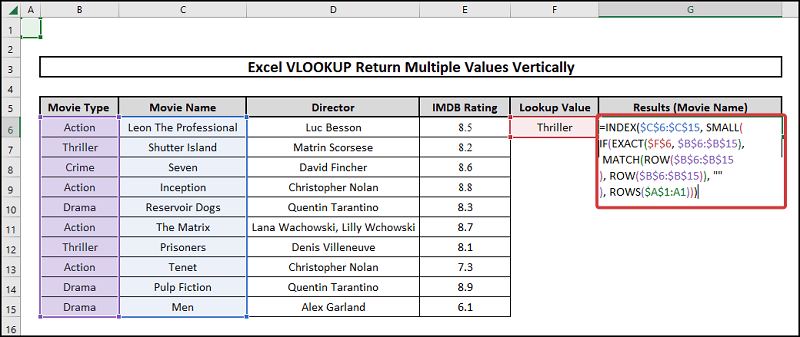
2. INDEX-MATCH with EXACT Function
Here we will be using a combination of different functions to filter out movie lists vertically. Therefore we will use INDEX, SMALL, EXACT, IF, MATCH, ROW, and ROWS functions
⬇️⬇️ STEPS ⬇️⬇️
- To start, copy down the following formula.
=INDEX($C$6:$C$15, SMALL(IF(EXACT($F$6, $B$6:$B$15), MATCH(ROW($B$6:$B$15), ROW($B$6:$B$15)), “”), ROWS($A$1:A1)))
🔨 Formula Breakdown
👉 EXACT($F$6, $B$6:$B$15)
Determines if the items in the array $B$6:$B$15 satisfy criterion $F$6=Thriller.
👉 MATCH(ROW($B$6:$B$15), ROW($B$6:$B$15))
MATCH function finds the relative position of multiple values.
👉 ROW($B$6:$B$15)
Using a cell reference as its basis, the ROW function returns the row number.
👉 IF(EXACT($F$6, $B$6:$B$15), MATCH(ROW($B$6:$B$15), ROW($B$6:$B$15)), “”)
This part tells what to show if the criteria are satisfied and what if not satisfied
👉 SMALL(IF(EXACT($F$6, $B$6:$B$15), MATCH(ROW($B$6:$B$15), ROW($B$6:$B$15)), “”), ROWS($A$1:A1))
Row numbers are filtered using the SMALL function from smallest to largest. Here ROWS($A$1:A1) is used to get the number 1.
👉 INDEX($C$6:$C$15, SMALL(IF(EXACT($F$6, $B$6:$B$15), MATCH(ROW($B$6:$B$15), ROW($B$6:$B$15)), “”), ROWS($A$1:A1)))
The INDEX function provides a value in accordance with a cell reference and the column and row numbers. Therefore the reference here is $C$6:$C$15.
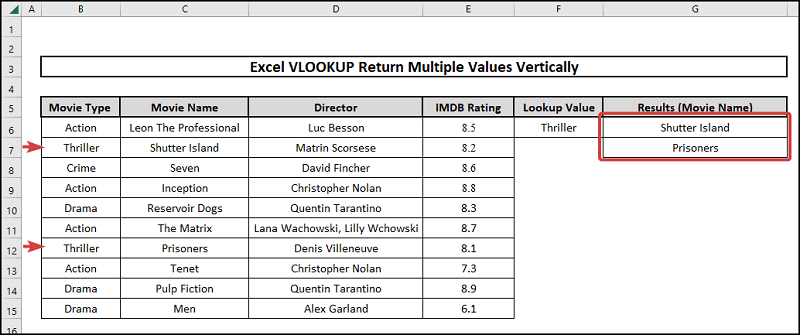
👉 Output– Shutter Island.
- After that, press Enter and copy down the formula for the results.
📕 Read More: What Is Table Array in VLOOKUP in Excel?
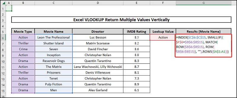
3. INDEX-MATCH with IF Function
In this method, we are going to use a series of functions to create a formula and determine the Action movie list. Therefore we will be using INDEX, SMALL, IF, MATCH, ROW, and ROWS functions.
⬇️⬇️ STEPS ⬇️⬇️
- Firstly copy down the following formula.
=INDEX($C$6:$C$15, SMALL(IF(($F$6=$B$6:$B$15), MATCH(ROW($B$6:$B$15), ROW($B$6:$B$15)), “”),ROWS($A$1:A1)))
🔨 Formula Breakdown
👉 ($F$6=$B$6:$B$15)
Determines if the items in the array $B$6:$B$15 satisfy criterion $F$6=Action.
👉 MATCH(ROW($B$6:$B$15), ROW($B$6:$B$15))
MATCH function finds the relative position of multiple values.
👉 ROW($B$6:$B$15)
Using a cell reference as its basis, the ROW function returns the row number.
👉 IF(($F$6=$B$6:$B$15), MATCH(ROW($B$6:$B$15), ROW($B$6:$B$15)), “”)
This part tells what to show if the criteria are satisfied and what, if not satisfied.
👉 SMALL(IF(($F$6=$B$6:$B$15), MATCH(ROW($B$6:$B$15), ROW($B$6:$B$15)), “”),ROWS($A$1:A1))
Row numbers are filtered using the SMALL function from smallest to largest. Here ROWS($A$1:A1) is used to get the number 1.
👉 INDEX($C$6:$C$15, SMALL(IF(($F$6=$B$6:$B$15), MATCH(ROW($B$6:$B$15), ROW($B$6:$B$15)), “”),ROWS($A$1:A1)))
The INDEX function provides a value in accordance with a cell reference and the column and row numbers. Therefore the reference here is $C$6:$C$15.
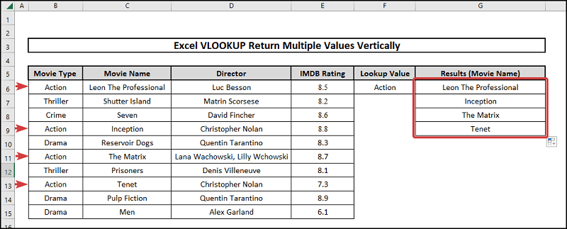
👉 Output– Leon The Professional.
- After that press Enter and copy down the formula for the results.
📕 Read More: 6 Solutions If VLOOKUP Returns #N/A When Match Exists in Excel
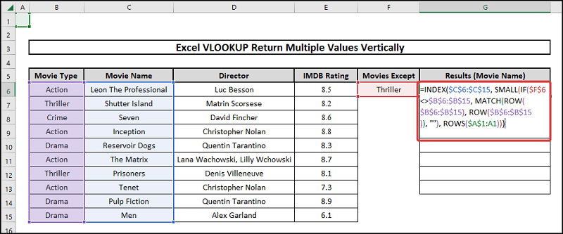
4. INDEX-MATCH to Vlookup Dissimilar Values
For instance say you want to watch a movie you have the dataset like us and you don’t like Thrillers. This is how you filter a movie list that is not Thrillers use this combination to demonstrate. Therefore we will be using INDEX, SMALL, IF, MATCH, ROW, and ROWS functions.
⬇️⬇️ STEPS ⬇️⬇️
- First copy down the following formula or modify it as per your data.
=INDEX($C$6:$C$15,SMALL(IF($F$6<>$B$6:$B$15,MATCH(ROW($B$6:$B$15),ROW($B$6:$B$15)), “”), ROWS($A$1:A1)))
🔨 Formula Breakdown
👉 $F$6<>$B$6:$B$15
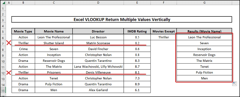
Determines if the items in the array $B$6:$B$15 is not equal to cell $F$6=Thriller.
👉 MATCH(ROW($B$6:$B$15), ROW($B$6:$B$15))
MATCH function finds the relative position of multiple values.
👉 ROW($B$6:$B$15)
Using a cell reference as its basis, the ROW function returns the row number.
👉 IF($F$6<>$B$6:$B$15,MATCH(ROW($B$6:$B$15),ROW($B$6:$B$15)), “”)
This part tells what to show if the criteria are satisfied and what, if not satisfied.
👉 SMALL(IF($F$6<>$B$6:$B$15,MATCH(ROW($B$6:$B$15),ROW($B$6:$B$15)), “”), ROWS($A$1:A1))
Row numbers are filtered using the SMALL function from smallest to largest. Here ROWS($A$1:A1) is used to get the number 1.
👉 INDEX($C$6:$C$15,SMALL(IF($F$6<>$B$6:$B$15,MATCH(ROW($B$6:$B$15),ROW($B$6:$B$15)), “”), ROWS($A$1:A1)))
The INDEX function provides a value in accordance with a cell reference and the column and row numbers. Therefore the reference here is $C$6:$C$15.
👉 Output– Leon The Professional.
- Press Enter and copy down the formula for the results.
📕 Read More: 5 Ways to Extract Filtered Data into Another Excel Sheet
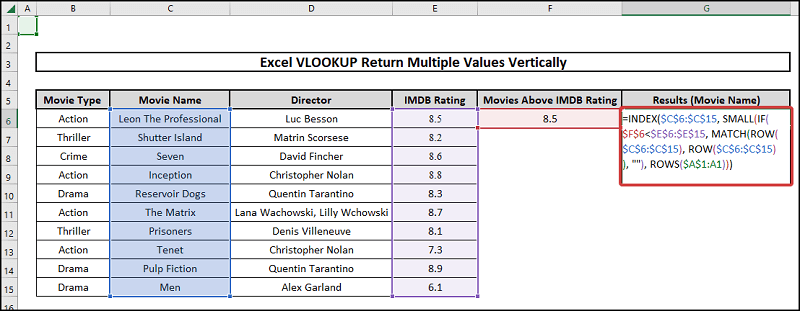
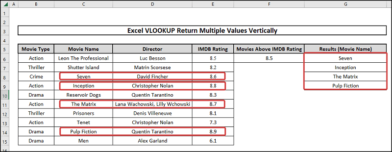
5. INDEX-MATCH to Vlookup Larger Values
Here we are going to use a combination of functions to determine values if a certain column is smaller than a criterion. Therefore we will be using INDEX, SMALL, IF, MATCH, ROW, and ROWS functions.
⬇️⬇️ STEPS ⬇️⬇️
- Firstly copy down the following formula or modify it according to your problem.
=INDEX($C$6:$C$15,SMALL(IF($F$6<$E$6:$E$15,MATCH(ROW($C$6:$C$15),ROW($C$6:$C$15)), “”), ROWS($A$1:A1)))
🔨 Formula Breakdown
👉 $F$6<$E$6:$E$15
Determines if the items in the array $E$6:$E$15 is larger than cell $F$6=8.5.
👉 MATCH(ROW($C$6:$C$15),ROW($C$6:$C$15))
MATCH function finds the relative position of multiple values.
👉 ROW($C$6:$C$15)
Using a cell reference as its basis, the ROW function returns the row numbers.
👉 (IF($F$6<$E$6:$E$15,MATCH(ROW($C$6:$C$15),ROW($C$6:$C$15)), “”)
This part tells what to show if the criteria are satisfied and what, if not satisfied.
👉 SMALL(IF($F$6<$E$6:$E$15,MATCH(ROW($C$6:$C$15),ROW($C$6:$C$15)), “”), ROWS($A$1:A1))
Row numbers are filtered using the SMALL function from smallest to largest. Here ROWS($A$1:A1) is used to get the number 1.
👉 INDEX($C$6:$C$15,SMALL(IF($F$6<$E$6:$E$15,MATCH(ROW($C$6:$C$15),ROW($C$6:$C$15)), “”), ROWS($A$1:A1)))
The INDEX function provides a value in accordance with a cell reference and the column and row numbers. Therefore the reference here is $C$6:$C$15.
👉 Output– Seven.
- After that press Enter and copy down the formula to get the answers.
📕 Read More: VLOOKUP to Find Duplicates in Two Columns in Excel
6. INDEX-MATCH to Vlookup Smaller Values
Here we are going to use a combination of functions to determine values if a certain column is smaller than a criterion. Therefore we will be using INDEX, SMALL, IF, MATCH, ROW, and ROWS functions.
⬇️⬇️ STEPS ⬇️⬇️
- Firstly copy down the following formula or modify it according to your problem.
=INDEX($C$6:$C$15,SMALL(IF($F$6>$E$6:$E$15,MATCH(ROW($C$6:$C$15),ROW($C$6:$C$15)), “”), ROWS($A$1:A1)))
🔨 Formula Breakdown
👉 $F$6>$E$6:$E$15
Determines if the items in the array $E$6:$E$15 is less than cell $F$6=8.5.
👉 MATCH(ROW($C$6:$C$15),ROW($C$6:$C$15))
MATCH function finds the relative position of multiple values.
👉 ROW($C$6:$C$15)
Using a cell reference as its basis, the ROW function returns the row numbers.
👉 (IF($F$6>$E$6:$E$15,MATCH(ROW($C$6:$C$15),ROW($C$6:$C$15)), “”)
This part tells what to show if the criteria are satisfied and what, if not satisfied.
👉 SMALL(IF($F$6>$E$6:$E$15,MATCH(ROW($C$6:$C$15),ROW($C$6:$C$15)), “”), ROWS($A$1:A1))
Row numbers are filtered using the SMALL function from smallest to largest. Here ROWS($A$1:A1) is used to get the number 1.
👉 INDEX($C$6:$C$15,SMALL(IF($F$6>$E$6:$E$15,MATCH(ROW($C$6:$C$15),ROW($C$6:$C$15)), “”), ROWS($A$1:A1)))
The INDEX function provides a value in accordance with a cell reference and the column and row numbers. Therefore the reference here is $C$6:$C$15.
👉 Output– Shutter Island.

- Press Enter and copy down the formula for the results.
📕 Read More: VLOOKUP to Find Duplicates in Two Columns in Excel
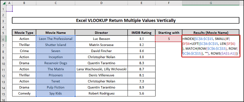
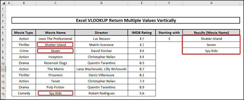
7. INDEX-MATCH to Vlookup Values Starting with Letter
For instance we want the movies’ list that starts with the letter S. Therefore, we are going to use INDEX, SMALL, IF, MATCH, LEN, LEFT, ROW, and ROWS functions.
⬇️⬇️ STEPS ⬇️⬇️
- Firstly copy the following formula.
=INDEX($C$6:$C$15,SMALL(IF($F$6=LEFT($C$6:$C$15,LEN($F$6)),MATCH(ROW($C$6:$C$15), ROW($C$6:$C$15)), “”), ROWS($A$1:A1)))
🔨 Formula Breakdown
👉 LEN($F$6)
Determines the length of the string which is 1.
👉 LEFT($C$6:$C$15,LEN($F$6))
The first character of the string $C$6:$C$15.
👉 $F$6=LEFT($C$6:$C$15,LEN($F$6))
This command sets the criteria being the first letter of string $C$6:$C$15 should be S.
👉 MATCH(ROW($C$6:$C$15),ROW($C$6:$C$15))
MATCH function finds the relative position of multiple values.
👉 ROW($C$6:$C$15)
Using a cell reference as its basis, the ROW function returns the row numbers.
👉 IF($F$6=LEFT($C$6:$C$15,LEN($F$6)),MATCH(ROW($C$6:$C$15),ROW($C$6:$C$15)), “”)
This part tells what to show if the criteria are satisfied and what, if not satisfied.
👉 SMALL(IF($F$6=LEFT($C$6:$C$15,LEN($F$6)),MATCH(ROW($C$6:$C$15), ROW($C$6:$C$15)), “”), ROWS($A$1:A1))
Row numbers are filtered using the SMALL function from smallest to largest. Here ROWS($A$1:A1) is used to get the number 1.
👉 INDEX($C$6:$C$15,SMALL(IF($F$6=LEFT($C$6:$C$15,LEN($F$6)),MATCH(ROW($C$6:$C$15), ROW($C$6:$C$15)), “”), ROWS($A$1:A1)))
The INDEX function provides a value in accordance with a cell reference and the column and row numbers. Therefore the reference here is $C$6:$C$15.
👉 Output– Shutter Island.
- After that press Enter and copy down the formula for the results.
📕 Read More: 3 Quick Ways to Vlookup and Return Multiple Values Horizontally
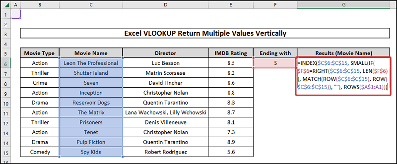
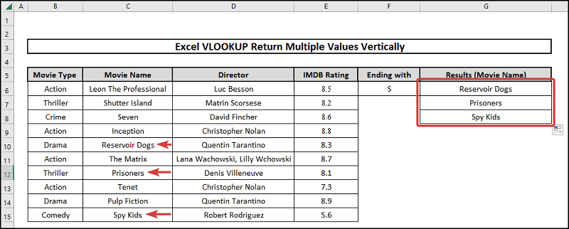
8. INDEX-MATCH to Vlookup Values Ending with Letter
For instance we want the movies’ list that ends with the letter S. Therefore, we are going to use INDEX, SMALL, IF, MATCH, LEN, RIGHT, ROW, and ROWS functions.
⬇️⬇️ STEPS ⬇️⬇️
- Firstly copy the following formula.
=INDEX($C$6:$C$15,SMALL(IF($F$6=RIGHT($C$6:$C$15,LEN($F$6)),MATCH(ROW($C$6:$C$15), ROW($C$6:$C$15)), “”), ROWS($A$1:A1)))
🔨 Formula Breakdown
👉 LEN($F$6)
Determines the length of the string which is 1.
👉 RIGHT($C$6:$C$15,LEN($F$6))
Last character of the string $C$6:$C$15.
👉 $F$6=RIGHT($C$6:$C$15,LEN($F$6))
This command sets the criteria being the last letter of string $C$6:$C$15 should be S.
👉 MATCH(ROW($C$6:$C$15),ROW($C$6:$C$15))
MATCH function finds the relative position of multiple values.
👉 ROW($C$6:$C$15)
Using a cell reference as its basis, the ROW function returns the row numbers.
👉 IF($F$6=RIGHT($C$6:$C$15,LEN($F$6)),MATCH(ROW($C$6:$C$15),ROW($C$6:$C$15)), “”)
This command tells what to show if the criteria are satisfied and what, if not satisfied.
👉 SMALL(IF($F$6=RIGHT($C$6:$C$15,LEN($F$6)),MATCH(ROW($C$6:$C$15), ROW($C$6:$C$15)), “”), ROWS($A$1:A1))
Row numbers are filtered using the SMALL function from smallest to largest and here ROWS($A$1:A1) is used to get the number 1.
👉 INDEX($C$6:$C$15,SMALL(IF($F$6=RIGHT($C$6:$C$15,LEN($F$6)),MATCH(ROW($C$6:$C$15), ROW($C$6:$C$15)), “”), ROWS($A$1:A1)))
The INDEX function provides a value in accordance with a cell reference and the column and row numbers. Therefore the reference here is $C$6:$C$15.
👉 Output– Shutter Island.
- After that press Enter and copy down the formula for the results.
📕 Read More: 7 Ways to Use VLOOKUP to Compare Two Lists
📄 Important Notes
🖊️ Be careful while using the code as there are a lot of terms and if you lose concentration the code may be incorrect.
🖊️ Use shortcuts to reduce time.
🖊️ Use Ctrl+Shift+Enter for arrays if you are not using Microsoft 365.
🖊️ While writing formulas carefully see the suggestions and don’t forget the commas and parentheses.
🖊️ Be careful while defining criteria to be accurate as the dataset.
🖊️ Use F4 for absolute values.
📝 Takeaways from This Article
📌 Firstly use of INDEX, MATCH, SMALL, IF, Exact, FILTER, ROW, and ROWS functions.
📌 How to VLOOKUP and return values vertically
📌 How to use multiple functions to create a formula.
📌 Determining multiple answers for given criteria.
Conclusion
Firstly, I hope you were able to use the techniques I demonstrated in this Excel VLOOKUP Return Multiple Values Vertically lesson. As you can see, there are a lot of options on how to do this decide deliberately on the approach that best addresses your circumstance. Moreover, I advise repeating the steps if you become confused in any of the steps if you get stuck. Practice on your own after taking a look at the Excel VLOOKUP Return Multiple Values Vertically Excel file in the practice workbook as I’ve provided above because practice makes a man perfect. Above all, I earnestly hope you can use it. Please share your experience with us in the comment box about how your experience was throughout the article and what we need to improve or add to make things better for you folks. However, if you have any problem regarding Excel spit it in the comment box. The Excelden crew is always available to answer your questions. In conclusion, keep educating yourself by reading. However, for more Excel-related articles please visit our website Excelden.com.
Related Articles
- Excel Formula: Use VLOOKUP Function with Multiple Sheets
- Find MAX of Multiple Values Using VLOOKUP Function in Excel
- 5 Examples to Use IF and VLOOKUP as Nested Function in Excel
- 2 Ways to Use VLOOKUP Function with Two Lookup Values


