If you have multiple columns and the columns contain duplicate values, this article will help you find those duplicates with ease. Today we will show you 9 simple ways of using VLOOKUP to find duplicates in two columns in Excel. I hope you will have fun reading the article.
📁 Download Excel File
Download this practice book to get deeper insight.
Overview of VLOOKUP Function
VLOOKUP is a search function that scans vertically across a table or spreadsheet for specific data. VLOOKUP is an abbreviation for vertical lookup. This function allows for approximate and exact matching, as well as wildcards (“*” or “?”) for partial matches. It requires lookup values to be in the first column of the table passed to it.
VLOOKUP function has the following syntax:
VLOOKUP(lookup_value, table_array, column_index_num, [range_lookup])
The arguments are:
lookup_value – The value to search for in a table’s first column.
table_array – The table from which a value is to be recovered.
column_index_num – The number of the table’s columns from which to recover a value.
range_lookup – TRUE for an approximate match. This is by default.
FALSE for the exact match.
📕 Read More: 8 Ways to VLOOKUP to Return Multiple Values Vertically in Excel
Learn to Use VLOOKUP to Find Duplicates in Two Columns in Excel Applying These 9 Methods
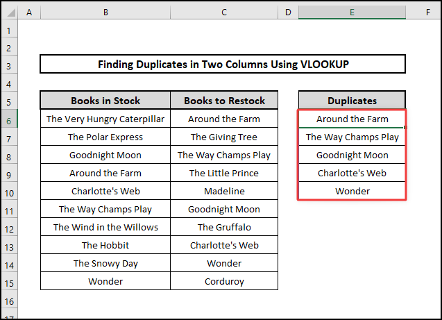
Today, to find duplicates in two columns in Excel, we will use not only VLOOKUP function but also the IFNA, IFERROR, ISERROR, ISNA, ISNUMBER, IF, FILTER, and finally, the MATCH function. We will make use of fictitious book store data that includes two columns of book lists. We will try to find duplicate books in those two columns. Let’s get to work.
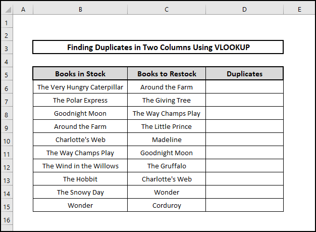
1. Using VLOOKUP Function
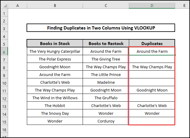
We will use VLOOKUP function to find only duplicates in this section. The ones that are not duplicates will show the #N/A error in the rows. Here are the steps to find duplicates in two columns using VLOOKUP in Excel.
⬇️⬇️ STEPS ⬇️⬇️
- First, enter this formula in cell D6.
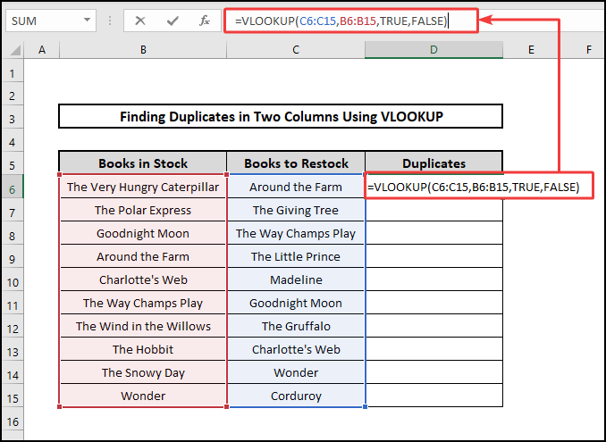
- Now, hit Enter, and the duplicate data in column D will be shown, along with a #N/A error if no match exists.
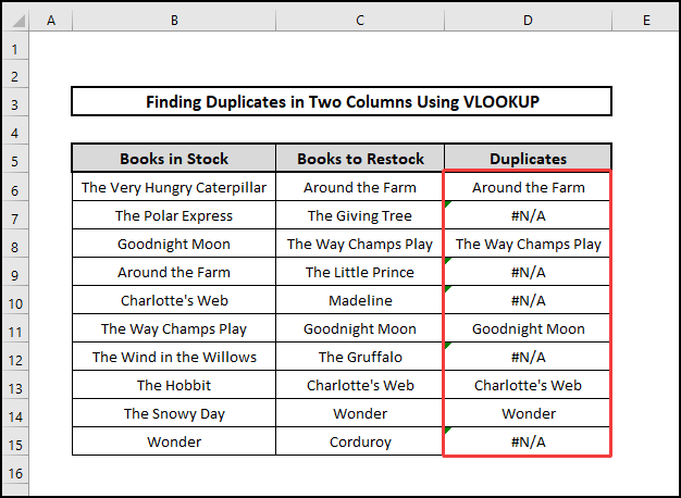
That’s it. You have completed the task you were assigned.
📕 Read More: 7 Ways to Use VLOOKUP to Compare Two Lists
2. Applying IFNA with VLOOKUP Functions
In the previous method, VLOOKUP showed #N/A when it found unique values. As a result, the table looked terrible. Therefore, if you want to eliminate those, you can work with the IFNA function. Let’s learn about the IFNA function.
Syntax of the IFNA function:
IFNA(value, value_if_na)
The arguments:
value – The parameter for which the #N/A error value is verified.
value_if_na – If the formula returns the #N/A error value, this value is returned.
If a formula produces the #N/A error value, the IFNA function returns the value you provide; otherwise, it returns the formula’s result.
⬇️⬇️ STEPS ⬇️⬇️
- First, select the cell you want to place your duplicate result. We are selecting cell D6 and writing this formula.
=IFNA(VLOOKUP(C6:C15,B6:B15 ,TRUE, FALSE),””)
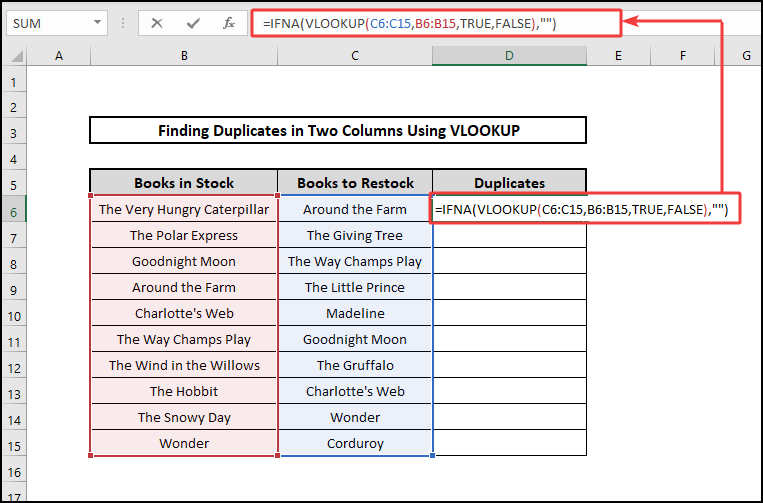
- Then, hit the Enter key, and the duplicate book names inside the two columns will be found.
As a result, you can see, the annoying #N/A errors have been omitted.
🔨 Formula Breakdown
👉 Like the 1st method, VLOOKUP produces #N/A error when it doesn’t find duplicates and prints the duplicate value when it does.
👉 Next, the IFNA function takes those # N/A errors and returns empty cells because in the formula we provided only “”.
📕 Read More: 6 Solutions If VLOOKUP Returns #N/A When Match Exists in Excel
3. Merging IFERROR with VLOOKUP Functions
The IFERROR function is an additional tool we can use in conjunction with VLOOKUP to find duplicates in Excel. The IFERROR function can be used to detect and manage faults in a calculation. If a formula evaluates to an error, IFERROR returns the value you specify; otherwise, it returns the formula’s result.
Syntax of IFERROR function:
IFERROR(value, value_if_error)
The arguments:
value – The value, reference, or formula that will be used to check for errors.
value_if_error – The value to return if there is an error.
Let’s write the formula in Excel.
⬇️⬇️ STEPS ⬇️⬇️
- First, select cell D6 and insert this formula in the Formula Bar.
=IFERROR(VLOOKUP(C6:C15,B6:B15,1,FALSE),””)
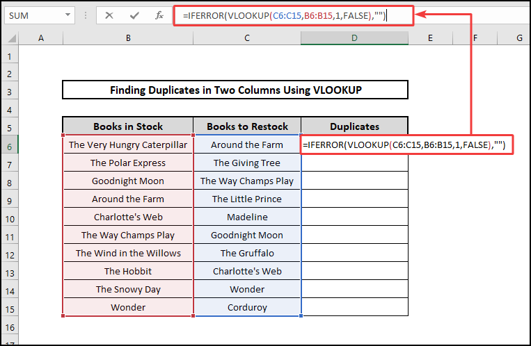
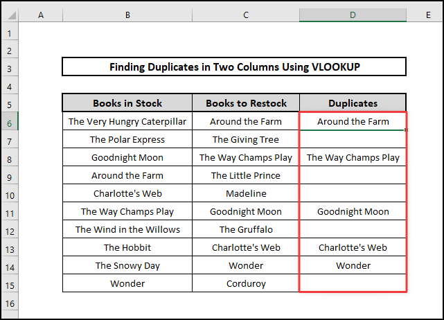
- Finally, press Enter to see the duplicates.
🔨 Formula Breakdown
👉 In the formula, VLOOKUP(C6:C15,B6:B15,1,FALSE) will look for duplicates in C6:C15 and return the duplicate values in D6:D15. When unable to find duplicates, it will return #N/A.
👉 Next, the IFERROR function will turn those #N/A into empty cells.
4. Combining of ISERROR and VLOOKUP Functions
Next in line is the ISERROR function, which can also be used with VLOOKUP to find duplicates in two columns in Excel. Excel’s ISERROR function will return TRUE for every error type, including #N/A and #VALUE!, #REF!, #DIV/0!, #NUM!, #NAME!, or otherwise #NULL! Hence, when an error occurs, you can check for issues, display a specific message, or run a fresh calculation by combining the ISERROR with IF function.
Syntax of the ISERROR function:
ISERROR(value)
Syntax of IF function:
IF(logical_test, value_if_true, [value_if_false])
The following arguments are required:
logical test – a logical phrase or value that may be evaluated as TRUE or FALSE.
value if true – When the logical test evaluates to TRUE, this value is returned.
value if false – When logical test returns FALSE, this value is returned.
⬇️⬇️ STEPS ⬇️⬇️
- First, to begin this procedure, go to cell D6 and enter the formula:
=IF(ISERROR(VLOOKUP(C6:C15,B6:B15,1,FALSE)),””,”Duplicate”)
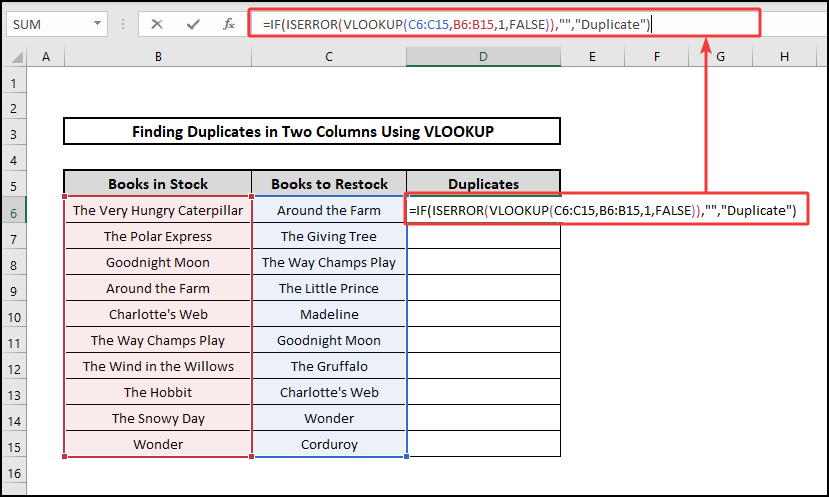
- Next, press Enter to see the term ‘Duplicates’ printed on the cells containing duplicate book names.
🔨 Formula Breakdown
👉 When duplicates are discovered, VLOOKUP prints the duplicate value instead of returning a #N/A error.
👉 Then, the ISERROR function returns FALSE for not finding the #N/A error in the first cell D6.
👉 Finally, IF returns ‘Duplicate’ for the FALSE return of the ISERROR function.
📕 Read More: 5 Examples to Use IF and VLOOKUP as Nested Function in Excel
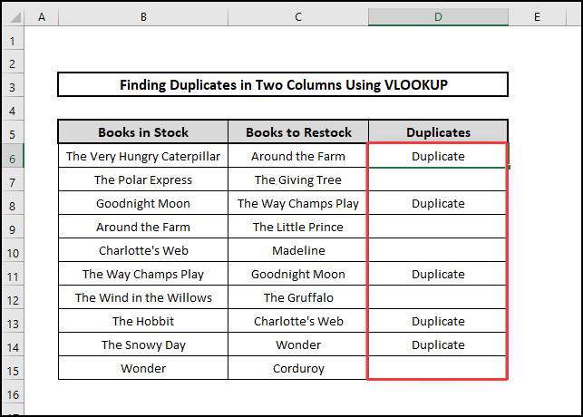
5. Utilizing ISNA with VLOOKUP Functions
The next function we will discuss is ISNA function. Besides, we will use the VLOOKUP and IF functions to find duplicates in two columns in Excel.
Syntax of ISNA function:
ISNA(value)
value – The value to test if there is #N/A.
When a cell has the #N/A error, ISNA returns TRUE, and it returns FALSE for every other value or error type.
⬇️⬇️ STEPS ⬇️⬇️
- First, select cell D6 and insert this formula.
=IF(ISNA(VLOOKUP(C6:C15,B6:B15,1,FALSE)),””,”Duplicate”)
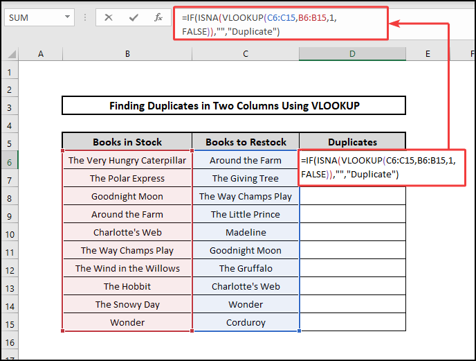
- Lastly, press Enter to see the result.
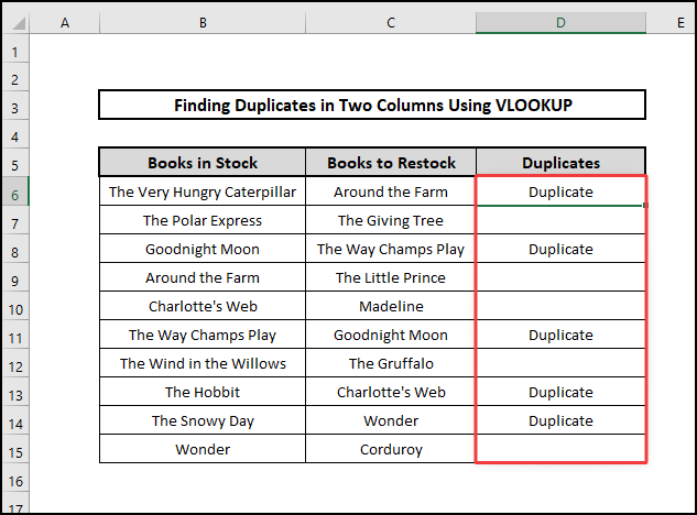
🔨 Formula Breakdown
👉 Instead of returning a #N/A error when duplicates are found, VLOOKUP prints the duplicate value.
👉 Then ISNA returns FALSE for duplicate values.
👉 Finally, IF will print ‘Duplicate’ for any FALSE declaration from ISNA and keep empty cells for any #N/A error.
6. Employing FILTER with VLOOKUP Function
If you want to avoid blank cells when VLOOKUP doesn’t find any duplicates, you can use FILTER function to clear the blank cells. We also use the IFNA function in this section.
FILTER function has the following syntax:
FILTER(array, include, [if_empty])
The arguments are:
array – The data range to filter.
include – the boolean array provided as criteria.
if_empty – value to return in the absence of results. This one is optional.
Based on specified criteria, FILTER function filters a set of data and retrieves matched entries.
⬇️⬇️ STEPS ⬇️⬇️
- First, in a separate cell E6, insert this formula.
=FILTER(C6:C15,IFNA(VLOOKUP(C6:C15,B6:B15,1,FALSE),””)<>””)
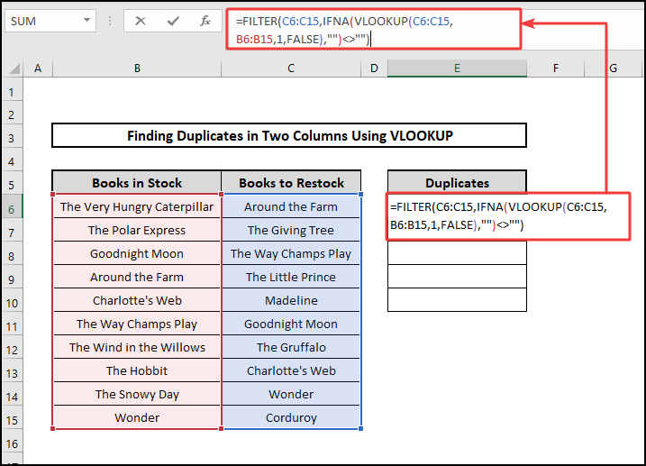
- Finally, press Enter to get only the duplicate values.
🔨 Formula Breakdown
👉 First, we give the lookup_value argument of VLOOKUP (C6:C15). The function compares each lookup_value to B6:B15, which returns an array of matches and #N/A errors for missing values.
👉 Second, the IFNA function replaces errors with empty strings before FILTER then filters out blanks (<>””) and outputs an array of matches as the final result.
📕 Read More: 5 Ways to Extract Filtered Data into Another Excel Sheet
7. Comparing Columns from Two Different Sheets
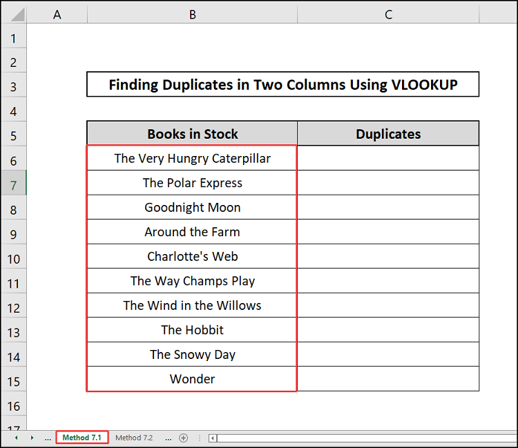
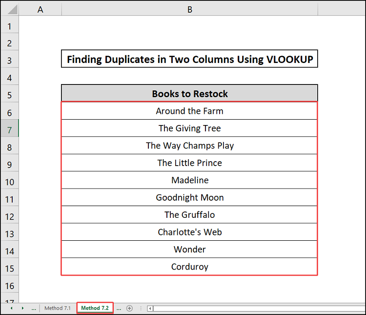
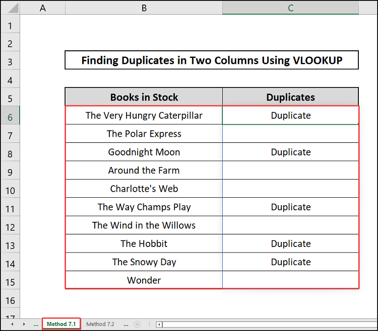
For this final technique, we’ll look at a unique scenario in which we might need to use VLOOKUP to find duplicates in two columns that reside in two different worksheets. For the sake of simplicity, we have named our worksheets Method 7.1 and Method 7.2, respectively. The idea is to take a set of data from Method 7.2 and compare it with the data from Method 7.1 to check for duplicates. For this section, we will use the IF, ISNA, and VLOOKUP functions.
Our Dataset in Method 7.1 worksheet.
And the dataset in Method 7.2 worksheet.
⬇️⬇️ STEPS ⬇️⬇️
- First, we will select our output cell located in Method 7.1 It is cell C6 and we shall insert the subsequent formula here.
=IF(ISNA(VLOOKUP(‘Method 7.2′!B6:B15,’Method 7.1’!B6:B15,1,FALSE)),””,”Duplicate”)
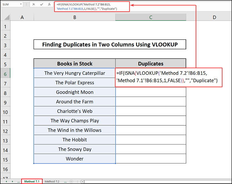
- To conclude, press Enter and see the magic.
🔨 Formula Breakdown
👉 First, in VLOOKUP, we put ‘Method 7.2′!B6:B15, to use the value as the lookup_value from the Method 7.2 worksheet and compare it with Method 7.1’!B6:B15.
👉 Next, ISNA returns FALSE for duplicate values.
👉 Finally, IF will print ‘Duplicate’ for any FALSE declaration from ISNA and keep empty cells for any #N/A error.
📕 Read More: Excel Formula: Use VLOOKUP Function with Multiple Sheets
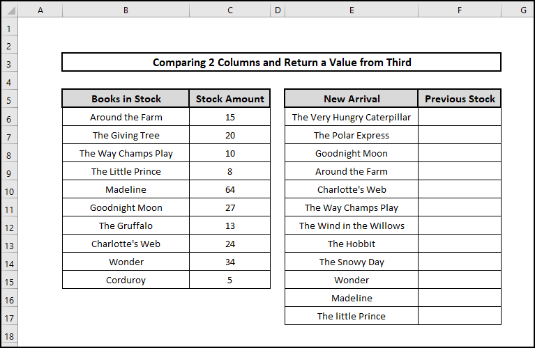
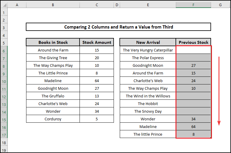
How to Compare Two Columns and Return a Value from Third Using Vlookup in Excel
You might occasionally have to compare two different columns from two distinct tables and then return a matched result based on another column while working with connected tables of data. In actuality, this is the main use of VLOOKUP function and the reason it was created. In this section, we will take data from different tables and bring them to the new one by comparing data from the old one. Like in this example, we have new arrival of the book collection and some of the books that arrived already existed in the previous slot. We will find out how many of them are left. To say it in Excel’s language, we will compare columns B and E and return values from C to F. We will use the IFNA and VLOOKUP functions here.
⬇️⬇️ STEPS ⬇️⬇️
- First, select F6 and write this formula.
=IFNA(VLOOKUP(E6,$B$6:$C$15,2,FALSE),””)
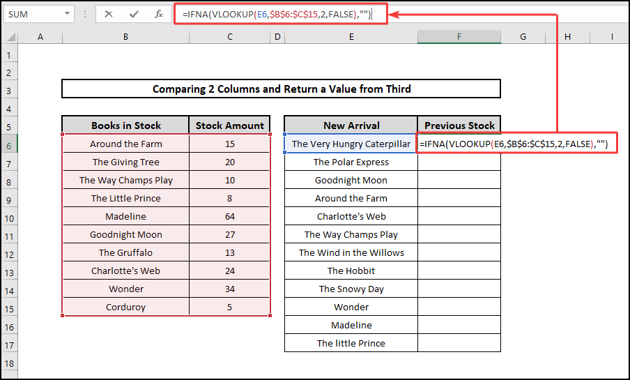
- Then, press Enter to see the results. As there is no match for E6 in $B$6:$C$15, it will show empty.
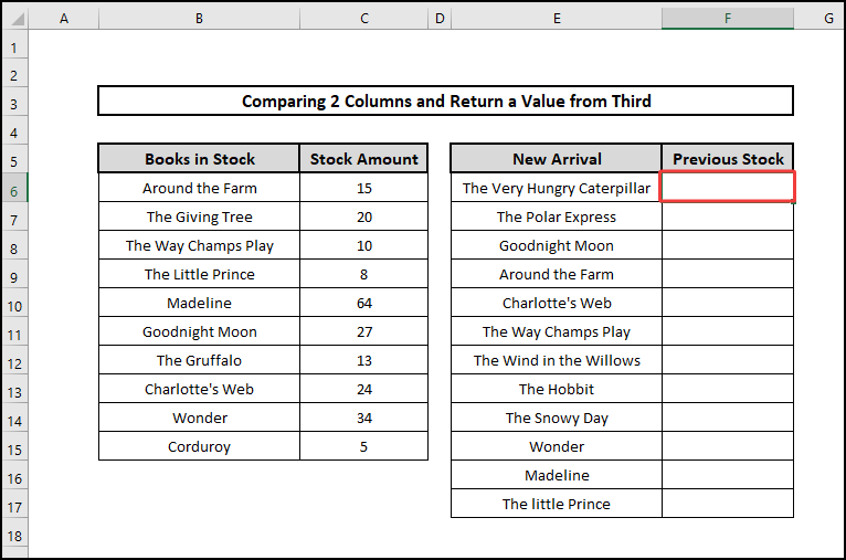
- Finally, hit the Fill Handle tool to copy the formula to the entire column.
🔨 Formula Breakdown
👉 First, the VLOOKUP will take the content of E6 and compare it to the contents of $B6:$C15.If it didn’t find any matches, it would return an #N/A error.
👉 Finally, the IFNA function would take that #N/A error and return a blank cell. When VLOOKUP matches anything, it will print data from column D.
📕 Read More: Find MAX of Multiple Values Using VLOOKUP Function in Excel
📝 Takeaways from This Article
📌 Putting TRUE in the column_index_num argument of VLOOKUP will act as the default value of the argument.
📌 To eradicate #N/A errors, we used IFNA and IFERROR functions with VLOOKUP.
📌 To print custom messages, we use the IF, ISNA, and ISERROR functions with VLOOKUP.
📌 We used FILTER to sort out only the duplicate values.
📌 We showed how users can compare duplicates in two different worksheets in Excel.
📌 Reading this article will help viewers to sort out duplicates and if needed, eliminate them
📌 This article will introduce readers to different functions to work on other projects.
Conclusion
So that’s it for today. Finally, we have come to the conclusion of our article. I hope I have described some easy ways to use VLOOKUP to find duplicates in two columns in Excel without complicating things too much. If you know another way to achieve the same result, feel free to comment below. For more tips and tricks for Excel, you are welcome to visit Excelden.com.


