Organizing data using various techniques is quite common in Microsoft Excel. Records are arranged in a tabular form here. In cases of data tracking, there are significant examples where duplicate data exist. Data analysts mostly evaluate this repetition to avoid data overlap. Multiple uses are there using this feature of Excel. This article will help you with seven ways to count duplicates in two columns in Excel. It is applicable for multiple cells in Excel and you can eventually modify it according to your requirements. All the methods have step-by-step instructions with a figurative description.
📁 Download Excel File
Download the Excel file below.
Learn to Count Duplicates in Two Columns in Excel with These 7 Approaches
The article is going to introduce seven approaches in Excel to count duplicates in two columns. The methods will help you understand the uses elaborately. The following discussion will cover the uses of the COUNTIF, SUMPRODUCT, MATCH, SUM, VLOOKUP, and ISNUMBER functions. You can also use the Filter feature to count duplicates in two columns by the SUBTOTAL function in Excel. Therefore, users will get a walkthrough of these solutions. A dataset will be modified in the following methods below to help you understand.

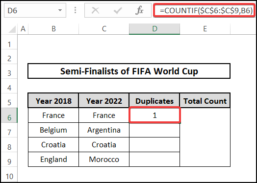
1. Applying COUNTIF and SUM Functions
To count duplicates in two columns in Excel, you can use the COUNTIF function. The SUM function is useful if you want to evaluate the total count.
⬇️⬇️ STEPS ⬇️⬇️
- Firstly, select cell D6.
- Secondly, enter the following formula.
- Thirdly, hit the Enter key.
- Fourth, copy the formulas down their cells using the Fill Handle icon.

- Fifth, select cell E6.
- Sixth, enter the following formula here.
- Seventh, hit the Enter key.

 Read More: 8 Ways to Count Duplicate Values in Multiple Columns in Excel
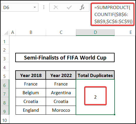
2. Utilizing SUMPRODUCT and COUNTIF Functions
The COUNTIF function can directly return the total amount of duplicates from two columns. For the process, you can take help from the SUMPRODUCT function.
⬇️⬇️ STEPS ⬇️⬇️
- Initially, select cell D6.
- Next, enter the following formula here.
- Then, hit the Enter key.
🔨 Formula Breakdown
SUMPRODUCT(COUNTIF($B$6:$B$9,$C$6:$C$9))
👉 Here, COUNTIF returns the cell numbers that have C6:C9 data from B6:B9.
👉 Also, SUMPRODUCT adds and multiplies returns from the COUNTIF function.
Finally, you get the total duplicate number as 2.
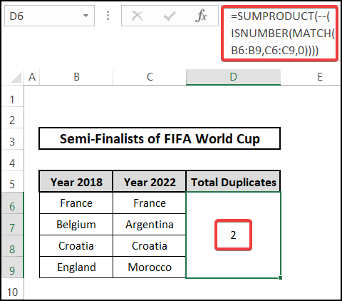
3. Employing MATCH and ISNUMBER Functions
You can match data range with the help of the MATCH function. To get duplicate counts from it, you can use the ISNUMBER function. Afterwards, the SUMPRODUCT function can return you the total number.
⬇️⬇️ STEPS ⬇️⬇️
- In the beginning, Initially, select cell D6.
- Now, enter the following formula here.
- After that, hit the Enter key.
🔨 Formula Breakdown
SUMPRODUCT(–(ISNUMBER(MATCH(B6:B9,C6:C9,0))))
👉 Here, MATCH looks for B6:B9 data range from data range C6 to C9. It returns the search value.
👉 Also, ISNUMBER returns the value from the MATCH function.
👉 Finally, SUMPRODUCT adds and multiplies returns from the ISNUMBER function.
Finally you get the total duplicate number as 2.
4. Merging SUM and MATCH Functions
The MATCH function can also be used with the SUM function to count the duplicates in two columns in Excel. For that, you can use the help from the IF function and the ISNA function.
⬇️⬇️ STEPS ⬇️⬇️
- To begin with, select cell D6.
- Here, enter the following formula here.
- Then, hit the Enter key.

🔨 Formula Breakdown
SUM(IF(ISNA(MATCH(B6:B9,C6:C9,0)),0,1))
👉 Here, MATCH looks for B6:B9 data range from data range C6 to C9. It returns the exact match value.
👉 Also, ISNA returns FALSE if there is no error. In case of an error, it returns TRUE.
👉 Again, IF returns 0 or 1 according to the condition from the ISNA function.
👉 Finally, SUM adds returns from the IF function.
Finally, you get the total duplicate number as 2.
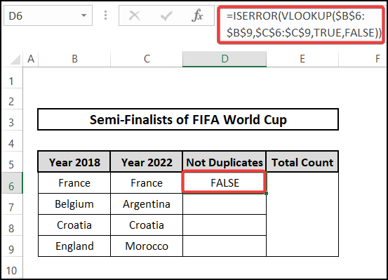
5. Utilizing VLOOKUP Function
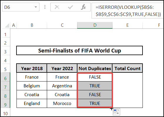
The VLOOKUP function is an important function to look for values and process appropriate actions regarding this. Using the ISERROR function can make sure that you don’t get error warning signs in the output. Finally, the COUNTIF function adds the results found.
⬇️⬇️ STEPS ⬇️⬇️
- Firstly, select cell D6.
- Secondly, enter the following formula.
- Thirdly, hit the Enter key.
- Fourth, copy the formulas down their cells using the Fill Handle icon.
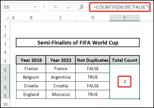
- Fifth, select cell E6.
- Sixth, enter the following formula here.
- Seventh, hit the Enter key.
🔨 Formula Breakdown
ISERROR(VLOOKUP($B$6:$B$9,$C$6:$C$9,TRUE,FALSE))
👉 Here, VLOOKUP looks for B6:B9 from cell range C6:C9.
👉 Furthermore, ISERROR refers to error value.
Finally you get the total duplicate number as 2.
6. Applying Filter with SUBTOTAL Function
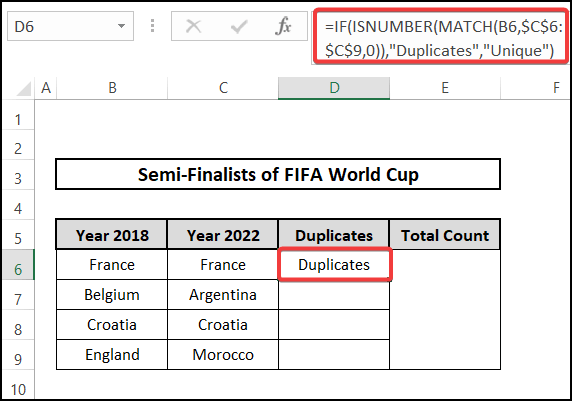
You can use the IF function along with the ISNUMBER and the MATCH functions to get “Duplicates” on the duplicate data and “Unique” otherwise. From the return, you can filter them based on duplicates. Finally, you should use the SUBTOTAL function to count the duplicates in two columns in Excel.
⬇️⬇️ STEPS ⬇️⬇️
- Initially, select cell D6.
- Next, enter the following formula here.
- Then, hit the Enter key.
- Now, copy the formulas down their cells using the Fill Handle icon.

- After that, select cell range D5:D9.
- Here, choose the Filter option from the Sort & Filter drop-down, under the Editing group of the Home tab.
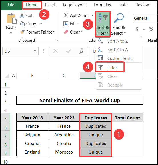
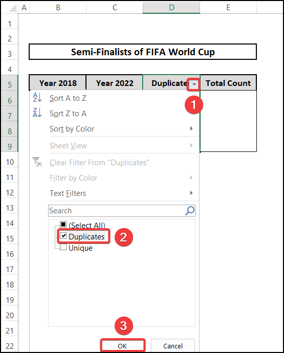
- Next, you will find a drop-down option available beside the column header like the following image.
- Then, click on the drop-down key.
- Now, choose only “Duplicates” from the filter options.
- After that, hit the OK option.
- Here, select cell E6.
- Now, enter the following formula here.
- Finally, hit the Enter key.
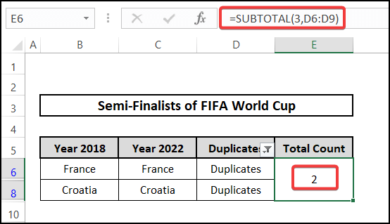
🔨 Formula Breakdown
IF(ISNUMBER(MATCH(B8,$C$6:$C$9,0)),”Duplicates”,”Unique”)
👉 Here, MATCH looks for B8 data range from data range C6 to C9. It returns the exact match value.
👉 Also, ISNUMBER returns the value from the MATCH function.
👉 Again, IF returns “Duplicates” or “Unique” according to the condition from ISNUMBER function.
Finally you get the total duplicate number as 2.
7. Counting Duplicates for Different Worksheet
The aforementioned six methods are applicable to datasets of the same worksheet. Now, if you want to count duplicates in two different columns from different worksheets in Excel, you can use the VLOOKUP, the ISERROR function, and the IF function.
⬇️⬇️ STEPS ⬇️⬇️
- In the beginning, select cell C6 from the worksheet “WC 2022”.
- Next, add the worksheet “WC 2018” with the formula.

- Then, complete the formula in the following way.

- Now, hit the Enter key.

- After that, copy the formulas down their cells using the Fill Handle icon.

- Next, select cell D6.
- Then, enter the following formula here.
- Finally, hit the Enter key.
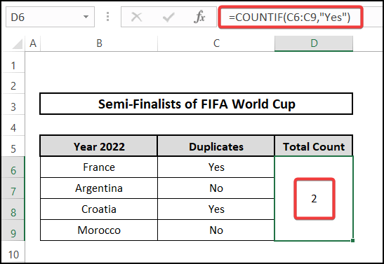
🔨 Formula Breakdown
IF(ISERROR(VLOOKUP(B6,’WC 2018′!$B$6:$B$9,1,0)),”No”,”Yes”)
👉 Here, VLOOKUP looks for B6 from cell range B6:B9 of worksheet “WC 2018”. The return gets to the ISERROR function.
👉 Furthermore, ISERROR refers to error value.
👉 Again, IF returns “No” or “Yes” according to the condition from ISERROR function.
Finally you get the total duplicate number as 2.
📄 Important Notes
🖊️ You should modify your formulas according to your dataset.
📝 Takeaways from This Article
The article lets the readers understand the variety of options available to count duplicates in two columns in Excel.
📌 Primarily, you can count duplicates in two columns using the COUNTIF and SUM functions in Excel.
📌 Also, you can use the SUMPRODUCT function with the COUNTIF function to count duplicates in two columns in Excel. You can directly get the totak numbers of duplicates.
📌 You can employ MATCH and ISNUMBER functions as well.
📌 Then, you can count duplicates in two columns using the SUM and MATCH functions in Excel. You should add IF and ISNA functions with it for better functionality.
📌 You can employ VLOOKUP functions as well.
📌 Also, you can use the Filter option with the SUBTOTAL function to count duplicates in two columns in Excel. You can directly get the total numbers of duplicates.
📌 Here, Excel can also count duplicates in two columns in two different worksheets.
Conclusion
To count duplicates in two columns in Excel, seven methods are useful. You can use the COUNTIF, SUMPRODUCT, MATCH, SUM, VLOOKUP, and ISNUMBER functions. The Filter feature with help of the SUBTOTAL function can help you with it as well. In case of further queries, readers are requested to leave a comment for the author. The author will try their best to come up with a suitable solution. Follow ExcelDen to get more access to solutions regarding your Excel problems.


