Are you struggling to find out sales data for a particular time? Different criteria under a certain period hit you hard? Then yes, you are on the right track; This is the perfect article for you. Use of SUMIF function in a data range link between two dates containing month as well as year. In this article, we will learn the use of the SUMIF function for the specific date range of month and year. Though the SUMIF function is only operatable under a single criterion. However, to allow multiple criteria, there is the SUMIFS function.
📁 Download Excel File
To practice please download the Excel file from here:
Learn to Use SUMIF in Date Range of Month and Year with These 11 Examples
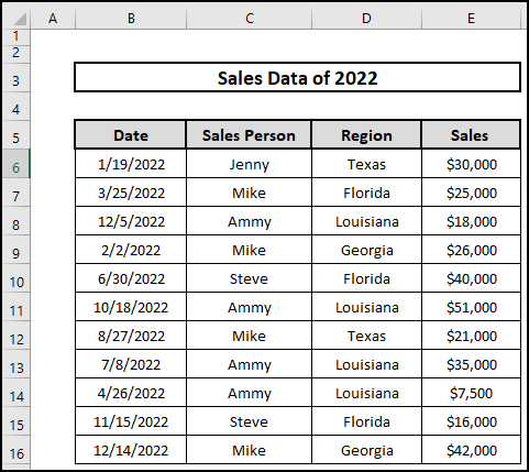
In this article, we are going to discuss 11 simple examples of to use of the SUMIF function in the specific date range of month and year. Here we consider a dataset named Sales Data of 2022 containing Date, Sales Person, Region, and Sales. There are 5 columns and 16 rows in the dataset. Later in this article, we are going to discuss the use of SUMIF, SUMIFS, SUM, IF, and SUMPRODUCT functions. In addition, the use of the Pivot table is also demonstrated. So, let’s get started.
1. Using SUMIF Function for Date Range of Specific Month and Year
SUMIF function usually sums up the values finding favorable data. Using the SUMIF function to define a particular month allows us to get that month’s sales data. Similarly, we can get sales data for a particular year. Please check out the below.
⬇️⬇️ STEPS ⬇️⬇️
- Initially, select a blank cell i.e. E18 to get the total sales.
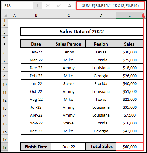
- Secondly, Insert the following formula in E18 containing the SUMIF function.
🔨 Formula Breakdown
👉 General logical expression: =SUMIF(range,”=”&cell,value_range)
👉 At first, C18= Dec-22 finds the date of december in B6:B16 range.
👉 After that, the SUMIF function gets the sales data for December month and sums up values.
- Therefore, we obtain the total sales of December 2022 at E18 which is $60,000.
 Read More: 3 Steps to Group Age Range in Excel Using VLOOKUP
2. Using SUMIF Function for Date Range of Less Than or Equal to a Month & Year
Suppose we need to determine total sales before July or till July; In this case, the SUMIF function is going to be our savior. Please follow the steps.
⬇️⬇️ STEPS ⬇️⬇️
- Primarily, select a blank cell i.e. E18 to get the total sales.
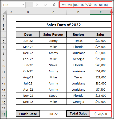
- Secondly, Insert the following formula in E18 containing the SUMIF function.
🔨 Formula Breakdown
👉 General logical expression: =SUMIF(range,”<“&cell, value_range)
👉 At first, C18 = Jul-22 finds the date before July in B6:B16 range.
👉 After that, the SUMIF function gets the sales data after July and sums up the values.
- Therefore, obtain the total sales before July 2022 at E18 which is $128,500.
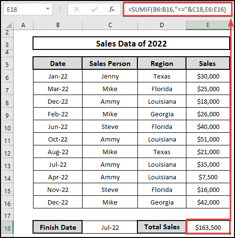
- Again use the following formula containing less than or less equal logical operation. Therefore, you will get the sales amount by July 2022.
3. Using SUMIF Function for Date Range of Greater Than or Equal to a Month & Year
Again if you are asked to determine total sales after July or from July, how are you going to find it out? In this case, the SUMIF function can save you once again. Please follow the steps.
⬇️⬇️ STEPS ⬇️⬇️
- Firstly, select a cell i.e. E18 to get the total sales.
- Secondly, Input the following formula in E18 having the SUMIF function.
🔨 Formula Breakdown
👉 General logical expression: =SUMIF(range,”>”&cell, value_range).
👉 At first, C18= Jul-22 finds the dates after July in B6:B16 range.
👉 After that, the SUMIF function gets the sales data after July and sums up the values.
- In the end, obtain the total sales of July to December 2022 at E18 which is $148,500.
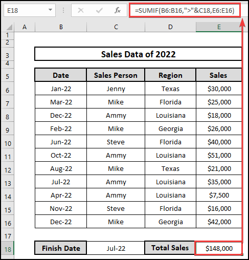
- Again use the following formula containing greater than or greater equal logical operation. Therefore, you will get the sales amount from July 2022.

4. Using SUMIF Function When Date Range Is Empty
You have a data sheet with some missing entry dates. To determine the total sales that are imputed without dates, follow the steps below.
⬇️⬇️ STEPS ⬇️⬇️
- Firstly, select a cell i.e. E18 to get the total sales that are without entry dates.
- Secondly, Remember in this case we need to keep empty cell E18.
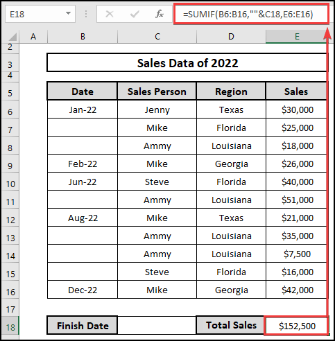
- Thirdly, Input the following formula in E18 having the SUMIF
🔨 Formula Breakdown
👉 General logical expression: =SUMIF(range,””&cell, value_range)
👉 At first, C18=[blank] finds the date of december in B6:B16 range.
👉 After that, the SUMIF function gets the sales data for December month and sums up values.
- Finally, Get the total sales of blank dates at E18 which is $152,500.
5. Using SUMIFS Function for a Given Date Range
SUMIF function generally runs under a certain criterion. On the other hand, to operate under multiple criteria, we need to use the SUMIFS function. Please follow the procedure below.
⬇️⬇️ STEPS ⬇️⬇️
- Initially, select a cell i.e. E18 to get the total sales that are without entry dates.
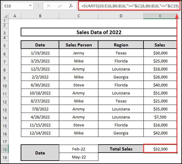
- Then, Input the following formula in E18 having the SUMIFS function for multiple criteria.
🔨 Formula Breakdown
👉 General logical expression: =SUMIFS(range_value, ,range,”>=”&lookup, range,”<=”&lookup)
👉 At first, the SUMIFS function finds C18 and C19 in B6:B16 which is between Feb-22 to May-22.
👉 After that, the SUMIF function gets the sales data and sums up values.
- Finally, Get the total sales between Feb-22 to May-22 at E18 which is $32,500.
6. Using SUMIFS and EOMONTH Functions
To find out the data of total sales in a specific month, SUMIFS along with the EOMONTH function can be a key to find it out. Please follow the steps below.
⬇️⬇️ STEPS ⬇️⬇️
- First, navigate a cell i.e. H6 to get the total sales in a specific month.
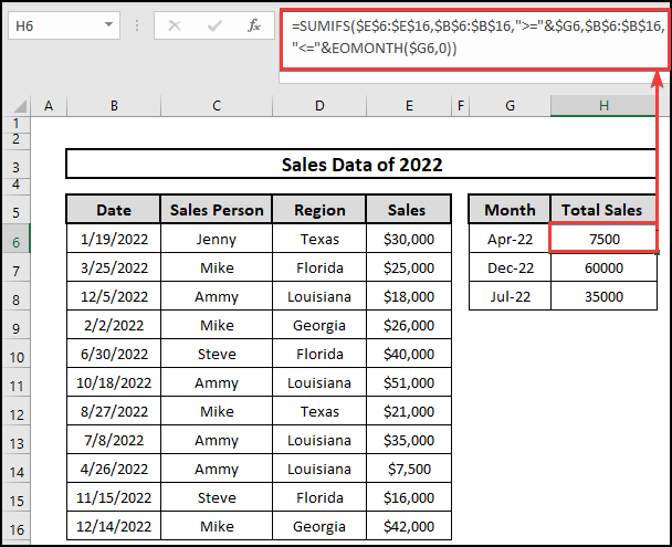
- Second, Input the following formula in H6 having the SUMIFS and EOMONTH functions to get the total sales in a month.
🔨 Formula Breakdown
👉 General logical expression: =SUMIFS(range_value,range,”>=”&lookup, range,”<=”&EOMONTH(lookup_data,0)
👉 At first, the SUMIFS function finds G6 in B6:B16 which is between Apr-22.
👉 Next, the EOMONTH function matches the month value to the B6:B16 range.
👉 After that, the SUMIF function gets the sales data and sums up values.
- Finally, Get the total sales at H-6, H-7, and H-8 respectively for Apr-22, Dec-22, and Jul-22.
7. Using SUMPRODUCT Function
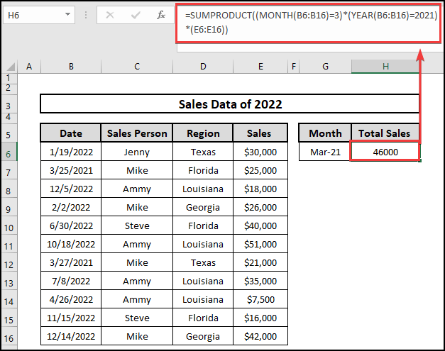
Suppose we need to find out the total sales for March 21. Here we can say, we have to match two different criteria one is the month, another is the year. To allow multiple criteria SUMPRODUCT can be another way to determine total sales in a specific time. Please follow the steps.
⬇️⬇️ STEPS ⬇️⬇️
- Initially, navigate a cell i.e. H6 to get the total sales in a specific month as well as year.
- Second, put the following formula in H6 having the SUMPRODUCT function to get the total sales in May 2021.
🔨 Formula Breakdown
The general syntax of the SUMPRODUCT function:
=SUMPRODUCT(array1, [array2], [array3], …)
👉 General logical expression: =SUMPRODUCT((MONTH(range)=3)*(YEAR(range)=2021)*(range_value)).
👉 (MONTH(B6:B16)=3; Here, 3=March that means find March from B6:B16 range.
👉 (YEAR(B6:B16)=2021) means find 2021 from B6:B16 range.
👉 After that, the SUMPRODUCT function gets the sales data and sums up the values of Mar-22.
- Lastly, Get the total sales of $46,000 at H-6 for Mar-21.
8. Summing Up Values for a Month of a Year Based on Criteria
Say, we need to find out the total sales of Jan-22 in Texas. The SUMIF function isn’t the way to count sales in this case. SUMIF function generally allows a criterion. On the other hand, to operate under multiple criteria, we need to use the SUMIFS function. Please follow the procedure below.
⬇️⬇️ STEPS ⬇️⬇️
- Primarily, select a cell i.e. H7 to get the total sales of Jan-22 in Texas.
- Then, Insert the following formula in H7 having the SUMIFS function for multiple criteria.
🔨 Formula Breakdown
👉 Here in this formula, B6:B16,”>=”&DATE(2022,1,1),B6:B16,”<=”&DATE(2022,1,31) is to select January month dated 1st to 31st.
👉 Following the date now it finds Texas in the D6:D16 range.
👉 After that, the SUMIF function gets the sales data for Texas at Jan-2022 and sums up values.
- Finally, Get the total sales of Jan-22 at H7 which is $30,000.

9. Using SUM and IF functions for a Month of a Year Based on Criteria
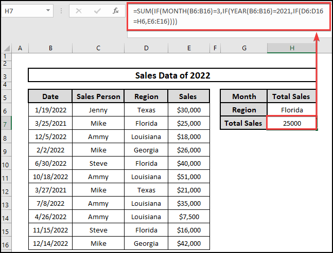
Let, we are asked to find out the total sales of March 21 in Florida. The SUM and IF functions combination can be a way to operate under multiple criteria instead of the SUMIFS function. Please follow the procedure below.
⬇️⬇️ STEPS ⬇️⬇️
- Primarily, select a cell i.e. H7 to get the total sales of Jan-22 in Texas.
- Then, Insert the following formula in H7 containing the SUM and IF function combination for multiple criteria.
🔨 Formula Breakdown
👉 Firstly in this formula, MONTH(B6:B16)=3 indicates to find 3rd month March in B6:B16 range using the MONTH function.
👉 Secondly, YEAR(B6:B16)=2021 dictates to find year 2021 in B6:B16 range using the YEAR function.
👉 Thirdly, D6:D16=H6 signals to find H6 = Florida in D6:D16 range.
👉 Fourthly, the IF function calls up the SUM function to add all the data.
- Finally, Get the total sales of Mar-21 in Florida at H7 which is $25,000.
10. Using Pivot Table Feature
Using the Pivot table we can easily find all the data separately. Please follow the necessary procedure.
⬇️⬇️ STEPS ⬇️⬇️
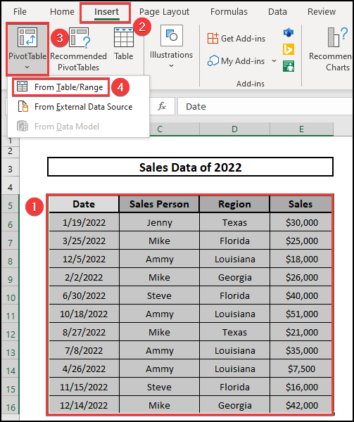
- First, select the entire range of the dataset.
- Then, from the Insert menu click on the Pivot Table feature.
- Next, from the Pivot Table dropdown box, select From Table/Range option.
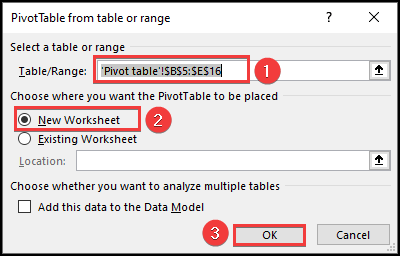
- Thus, a box named PivotTable from Table or range appears.
- Next, Type, ‘Pivot table’!$B$5:$E$16 in the Table/Range cell.
- Then, choose New worksheet to get the result and click on the OK button.
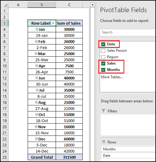
- On the right of the window, a PivotTable Fields section appears.
- Select the Date, Sales, and Months to get the values separately.
11. Sum Within a Dynamic Range Based on Today’s Date
Suppose, you are a marketing officer. Your duty is to collect dues. Say, there are dues of 30 days that haven’t been collected yet. To calculate the due of the past 30 days, please follow the steps below.
⬇️⬇️ STEPS ⬇️⬇️
- Primarily, select a cell i.e. H7 to get the dues.
- Then, Insert the following formula in H7 containing the SUMIFS function.
🔨 Formula Breakdown
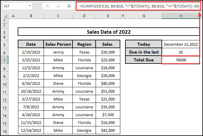
👉 Firstly in this formula, TODAY() delineates the date today means December 15, 2022.
👉 Secondly, B6:B16, “<“&TODAY(), B6:B16, “>=”&TODAY()-30 dictates finding dates past 30 days before today using the TODAY function.
👉 Finally, the SUMIFS function collects the values from the E6:E16 range and sums up values.
- Finally, there is two value Nov 15, 2022, and Dec 14, 2022. Summing these two values we get the final output at H7 which is $76,000.
📄 Important Notes
🖊️ Be careful and measure accurately during working with multiple formula combinations.
🖊️ Select the range of the dataset carefully during the use of the Pivot Table.
📝 Takeaway from This Article
📌 SUMIF function to sum up the values under a condition.
📌 EOMONTH function is dedicated to calling the data of that month.
📌 SUMIFS function allows multiple criteria whereas SUMIF only works under a single criterion.
📌 SUMPRODUCT function also works just like SUMIF in case of finding data from a range of months and years.
📌 Combination of SUM and IF functions also can be used just like the SUMIF function.
📌 Use of a Pivot Table also allows us to get the overall data separately.
Conclusion
We demonstrated every possible use of the SUMIF function in the data range of month and year in Excel. I hope you enjoyed your learning. Any suggestions, as well as queries, are appreciated. For better understanding and new knowledge don’t forget to visit www.ExcelDen.com.
Related Articles
- 4 Approaches to Capitalize All Letters in Excel Without Formula
- 7 Ways to Calculate Average Attendance with Formula in Excel
- 6 Quick Ways to Create Dynamic List from Table in Excel
- 7 Quick Ways to Calculate Average Percentage Increase in Excel


