When working with spreadsheets of large volumes, we often need to find and sort things properly. A drop down list is an efficient way of doing so and has lots of uses. Here, we will be discussing briefly about how we can link a cell value with a drop-down list in Excel by different approaches.
📁 Download Excel File
Download the Excel File below.
What Is a Drop-Down List?
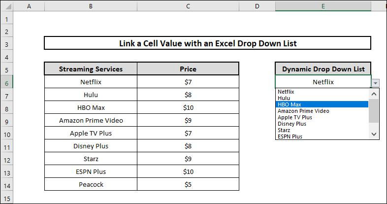
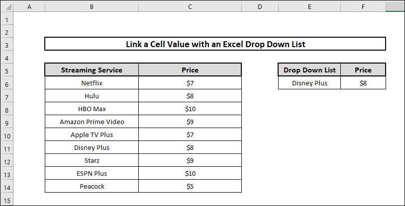
A drop down list can be defined as data validation function that allows us the users to choose an option from a list of choices. It is widely used in financial modelling and analysis. A drop down list looks like the following image:
Learn to Link a Cell Value with a Drop-Down List in Excel with These 5 Approaches
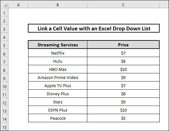
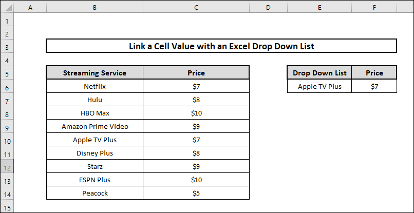
To demonstrate things clearly, we will be using a sample dataset to link a cell value with a Drop Down list in Excel in different approaches. Suppose that we have dataset of different online streaming services that are popular now and their monthly subscription rate. The dataset is shown as follows:
1. Using VLOOKUP Function
The syntax of the VLOOKUP Function is as follows:
Where lookup_value (Required) The required value we need to search for.
table_array (Required) The cells range where we need to search for the lookup value and look for a match.
column_index_num (Required) is the number of columns from which to return value.
Range_lookup (Optional) The number of columns from which the function needs to return a value.
We can use VLOOKUP Function to link a cell with a drop-down list. To do so, we have to follow the following steps:
⬇️⬇️ STEPS ⬇️⬇️
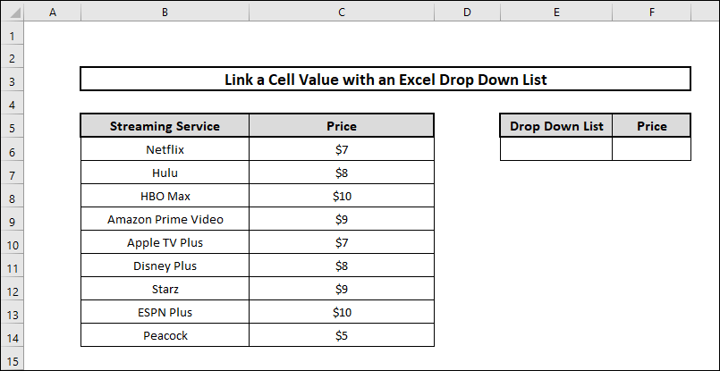
- First, we create two columns with the heading Drop Down List and Price.
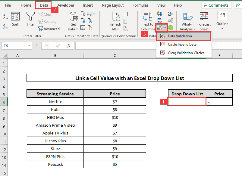
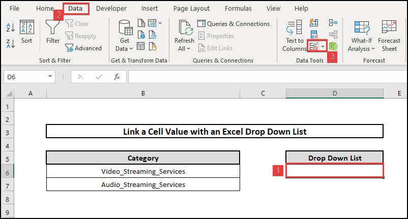
- We select cell E6 and then go to Data Validation from the Data Tools group.

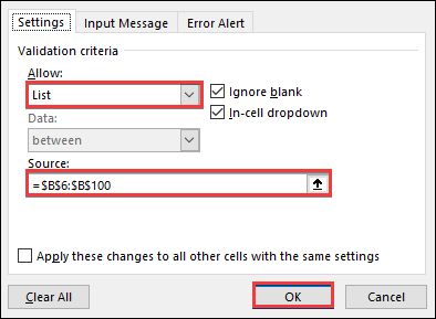
- A Data Validation box will appear. From the Validation Criteria, we select List from the Allow option, and in the Source box, we select the cells B6:B100 indicating the column Streaming Service.

- After that we press OK and we will see a drop-down list showing the entries of the Streaming services column.
- Now we move over to cell F6 and write the given formula in the formula bar and press Enter.
=VLOOKUP(E6,B5:C100,2,FALSE)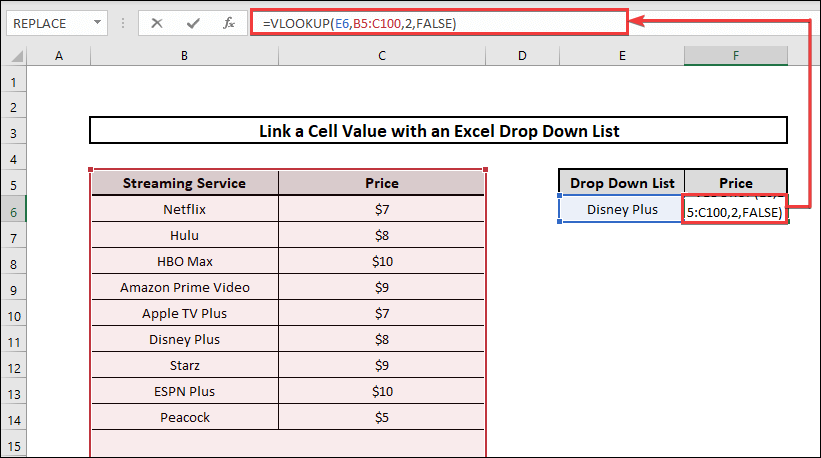
- Now we can see the corresponding price of the streaming service on the price column once we change the values of the streaming service in the drop-down list menu. The final results will be like the image below.
 Read More: 3 Ways to Create List from Range in Excel
2. Applying SUMIF Function
The syntax of the SUMIF function is as follows:
Where, range (Required) = The range of cells that we want to evaluate by a criteria.
criteria (Required) = the specification of which cells will be added, expressed as a number, expression, cell reference, text, or function.
Sum_range (Optional) = The actual range of cells to add if we want to add cells other than those specified in the range argument.
⬇️⬇️ STEPS ⬇️⬇️
- First, like the previous method, we make two columns with the headings Price and drop-down List.

- Then, we choose Data Validation from the Data Tools group after selecting cell E6.
- A box for data validation will show up. We choose List from the Validation Criteria’s Allow option, and in the Source box, we choose the cells B6 to B100 that represent the column Streaming Service.
- Once we select OK, a drop-down list with the entries from the Streaming services column will appear.
- For the next step, we proceed to cell F6 and enter the following formula in the formula bar.
=SUMIF(B5:B100,E6,C5:C100)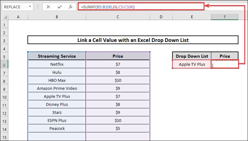
- Now as we change the streaming service’s values, the corresponding pricing change will appear in the price column. The result will look like the following image:
Read More: How to Create Drop-Down List in Multiple Columns in Excel
3. Utilizing Dynamic Drop-Down List
The Dynamic Drop-Down List is a great method because it allows us to update our data in the list with changes in the columns. To follow this step we are to do the following:
⬇️⬇️ STEPS ⬇️⬇️
- First, we create a column with the heading drop-down List.
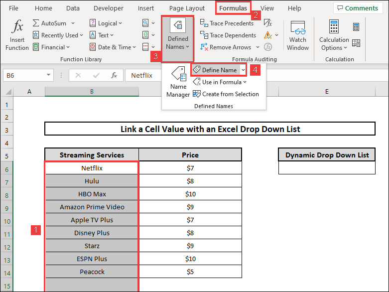
- After that, we select the cells B6:B100.
- Then we create a Named Selection by going to Formulas in the toolbar and then click Define Name.
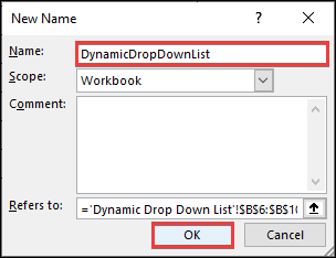
- A New Name box will appear and we write the selection name as DynamicDropDownList and press OK.
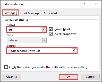
- Now, we select the cell E6 and then go to Data Validation from the Data Tools group.
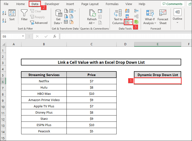
- We select List from the Validation Criteria Allow option and in the source option, we select the DynamicDropDownList and press OK.
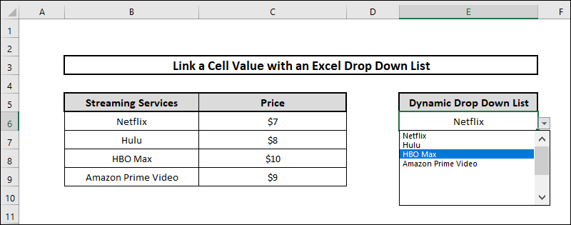
- The Drop Down list will be created like the following image.
- We can also check by adding or removing entries from the streaming services column. We will see that the Drop Down list will be updated continuously.
4. Using Dependent Drop-Down List
In this type of drop-down list, we need to make a list dependent upon another list. This drop-down list can also auto-update when there is a change in the dataset. To make a dependent drop-down list, we need to take the following steps:
⬇️⬇️ STEPS ⬇️⬇️
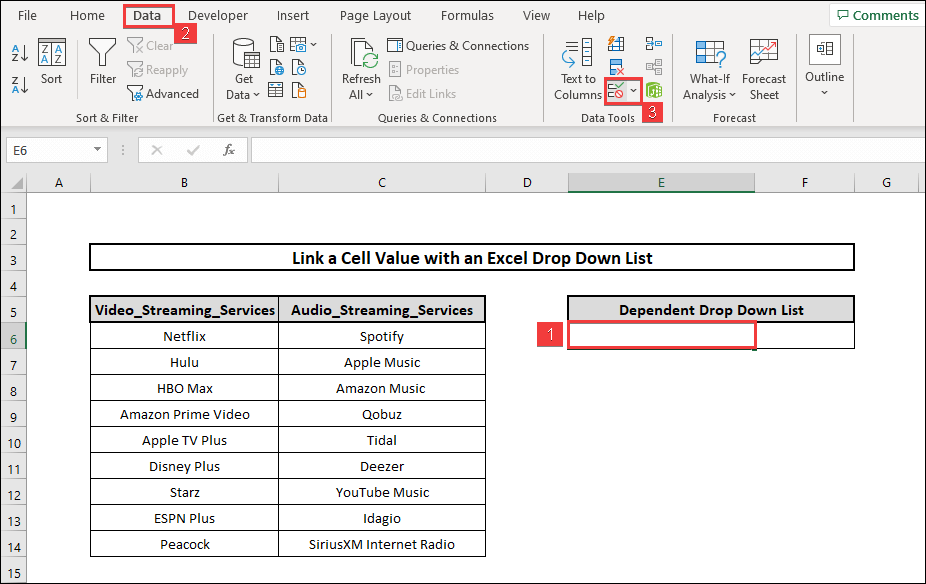
- First, we select cell E6 and go to Data Validation from Data Tools group in the Toolbar.
- A Data Validation box will appear. From the Allow option, we select List and in the source, we select the cells B5:C5 and press OK.
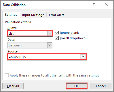
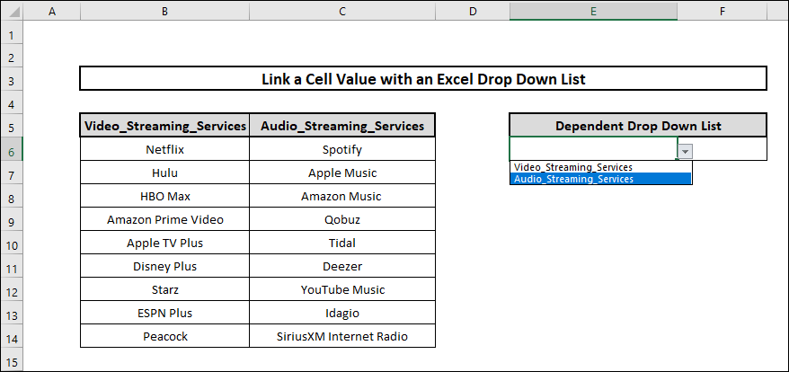
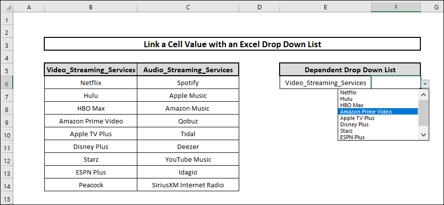
- A drop-down list will be created that features Video_Streaming_Services and Audio_Streaming_Services.
- Now we select the whole data range from B5:C14 and go to Formulas tab and click on Create from Selection.
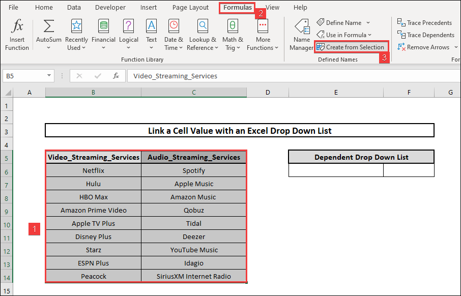
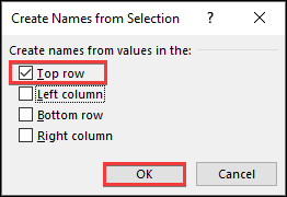
- A Create Names from the Selection box will appear where we check only the Top row and press OK. We can now go to Name Manager and see if a Name Selection has been created.
- Now we go to cell F6 and select Data Validation from the Data Menu.
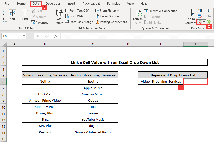
- In the Data Validation tab, we input the list in the Allow box, and in the source box, we write the following formula and press OK. We make sure that the cell does not have absolute reference.
=INDIRECT(E6)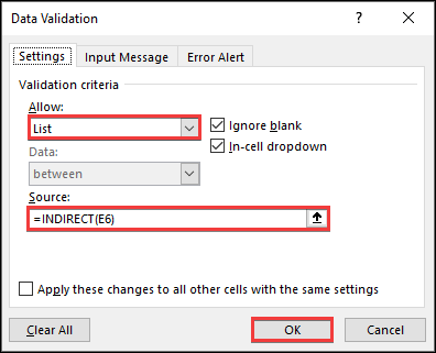
- The final results will appear as a drop-down menu dependent on another as in the image shown below.
5. Hyperlink Drop-Down List
In this method, we will use make a drop-down list that involves hyperlinking with separate worksheets. To do this, we need to follow these steps:
⬇️⬇️ STEPS ⬇️⬇️
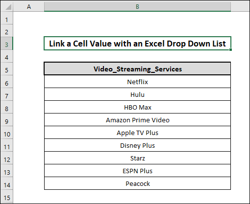
- First, we need to make two separate worksheets. We make one with the name Video_Streaming_Services.
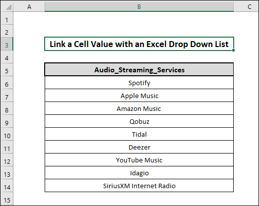
- After that, we make another worksheet named Audio_Streaming_Services.
- After that, we create another worksheet and make a category list of the two types of services. We write Video_Streaming_Services and Audio_Streaming_Services under this category section that we want to present as a drop-down list.
- We select cell D6 and make a drop-down list of the two categories by going to the Data Validation section from Data. After that we select List in the Allow field and in the source field we select the two category cell ranges B6:B7.
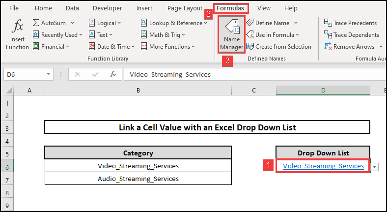
- Now we select D6, and then go to Formula and click Name Manager after that.
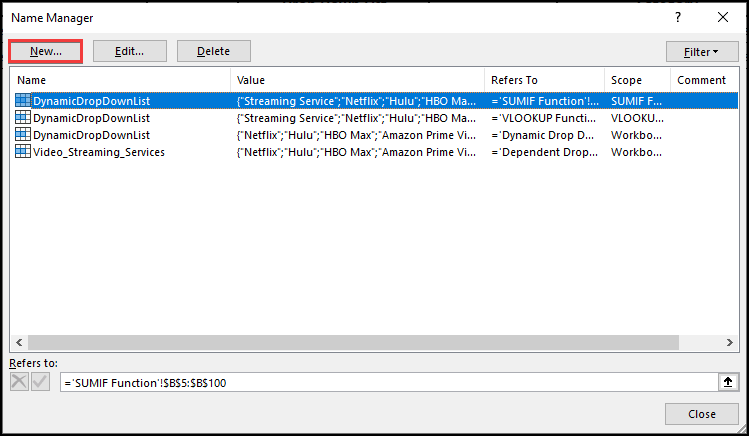
- We click on New in the Name Manager window.
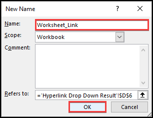
- A New Name box will appear. We fill the name box by writing Worksheet_Link and then we press OK.
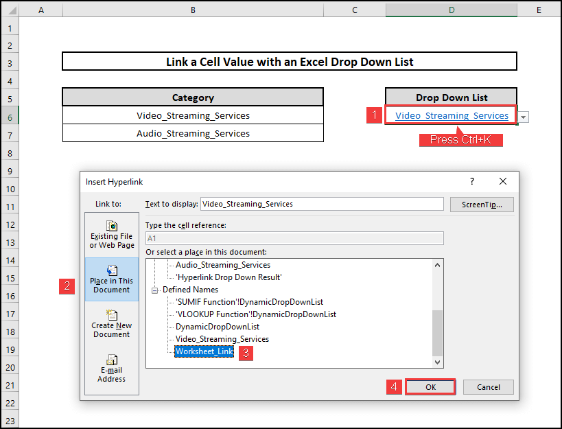
- After that, we select cell D6 and press Ctrl+K to insert the hyperlink in this cell. In this window, we select Place in This Document, click on Worksheet_Link and press OK.
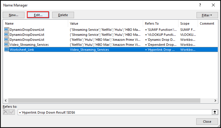
- Now we start to edit the hyperlink in cell D6. We select the cell, click on Formula, and then Name Manager.

- We select Worksheet_Link and then click on Edit on the Name Manager window.
- We write the following formula in the Refers to box and press OK.
=INDIRECT(ADDRESS(6,4,,,D6))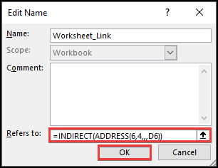
- Now, we have successfully created a hyperlink drop-down list. If we select any category now from the drop-down, we will go to that particular worksheet as these are hyperlinked. The results will be similar to the following image.
📄 Important Notes
🖊️ There can not be any spaces between characters while we are writing Named Range Names. Otherwise, Excel will not provide outputs as we desire. For Example, we have used underscores while writing two or more words such as Video_Streaming_Services.
🖊️ In the hyperlink drop-down list, the arguments of the ADDRESS Function [abs_num], [a1] are ignored and therefore we separated blank values with two commas (,,).
🖊️ When we are creating a dynamic drop-down list, we must keep in mind not to use absolute reference in cells like $D$6. We should use normal referencing like D6 instead.
📝 Takeaways from This Article
We have taken the following summed-up inputs from the article:
📌 We can make a drop-down list in Excel using Functions like VLOOKUP Function and SUMIF Function.
📌 We can also make a dynamic drop-down list and a dependent drop-down list that auto updates on the change in the dataset.
📌 Hyperlinking drop-down lists can be handy to use to separate sheets of an extensive database and access them easily.
Conclusion
In conclusion, this article has probably given you a complete idea about how you can link a cell value with a drop-down list in Excel. Feel free to ask any questions in the comment section if you want to. Follow our website ExcelDen to know more about Excel and its problems.


