4 Tricks to Show Zero Values in Pivot Table in Excel

Just think about a survey, where people don’t like to answer some particular question or they just avoid it. In this case, the cells for the particular question remain blank in the dataset. However, there is plenty of blank cells in the dataset. Some leave the data without making answers, some don’t like to answer or there are no activities to insert values. To make an overview in the pivot table, those cells of the dataset remain blank. So, sometimes we need to show zero values instead of blank cells in the pivot table. In this, we are going to learn several methods to show zero values in the pivot table.

Contents hide

📁 Download Excel File

Learn to Show Zero Values in Pivot Table in Excel with 4 Easy Approaches

1. Use Pivot Table Options to Replace Zero Values

2. Operate from Advanced Options to Insert Zero Values in Blanks

3. Use VBA Macro to Input Zero Values

4. Find Blanks and Insert Zero Values in Table

📄 Important Notes

📝 Takeaway from This Article

Conclusion

📁 Download Excel File

To practice please download the Excel file from here:

Pivot Table Show Zero Values.xlsm

Learn to Show Zero Values in Pivot Table in Excel with 4 Easy Approaches

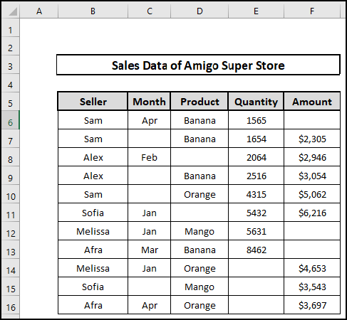
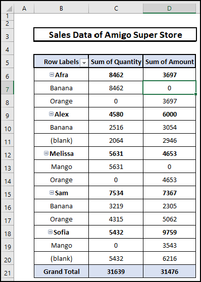
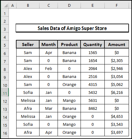
In this article, we explore 4 quick approaches to insert zero values in Pivot Table in Excel. Following that we considered a data set named Sales Data of Amigo Super Store- 2022 containing Seller, Month, Products, Quantity, and Amount. The dataset also has 16 rows and 6 columns including some blank cells. To insert zero values in Pivot Table, we are going to use the Pivot Table Options feature, Advance Option from Top Ribbon, and VBA Macro. Let’s get started.

method

1. Use Pivot Table Options to Replace Zero Values

Navigating the Pivot option from the Context Menu, one can easily insert zero values in the blank cells. But in this case, to get the pivot table option we need to make a pivot Table first. Please follow the steps below.

⬇️⬇️ STEPS ⬇️⬇️

Initially, select the total data range B5:F16.
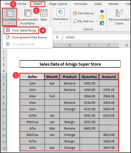
Secondly, to make a pivot table, click on the drop-down icon to pull down the list of Pivot Table from the Insert menu.
Thirdly, from the Pivot Table feature list, select From Table/ Range option.

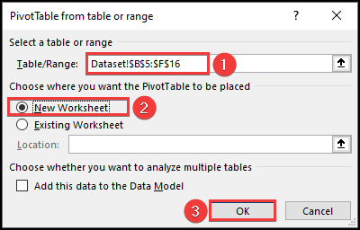
Now, a box named PivotTable from table or range appears.
Then, select $B$5:$F$16 for the table range cell from the Dataset worksheet.
Next, select Worksheet and hit the OK button.

Therefore we get the pivot table.
Then, click on Seller, Product, Quantity, and Amount appear.

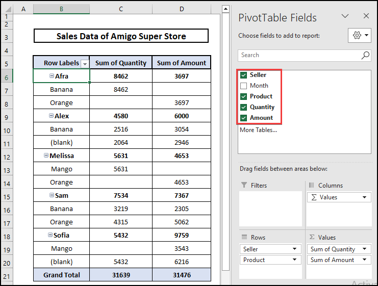
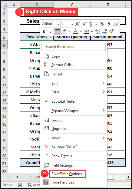
Again, select a cell i.e. B6.
Then, Right-Click on the mouse to get a Context Menu list.
Next, click on the PivotTable Options from the Context Menu list.

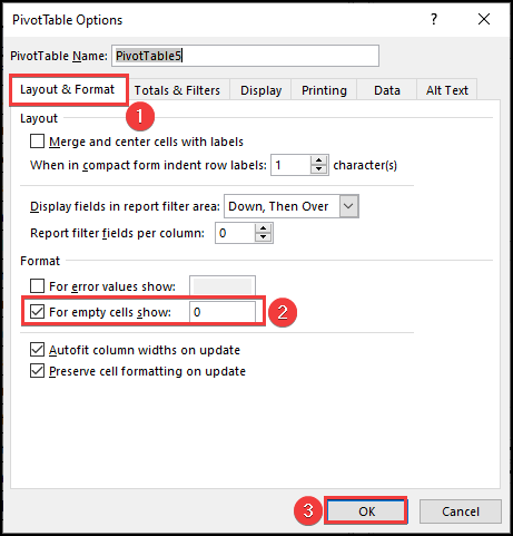
Thus, a box named PivotTable Options appears.
Further, from the Layout & Format option, insert 0 in For Empty Cells Show cell.
After that, click on the OK button.

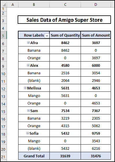
Finally, we observe the zero values in all the blank cells of the pivot table.

method

2. Operate from Advanced Options to Insert Zero Values in Blanks

From the File menu of Top Ribbon, one can easily insert zero values in the blank cells of a pivot table. Please follow the necessary procedure.

⬇️⬇️ STEPS ⬇️⬇️

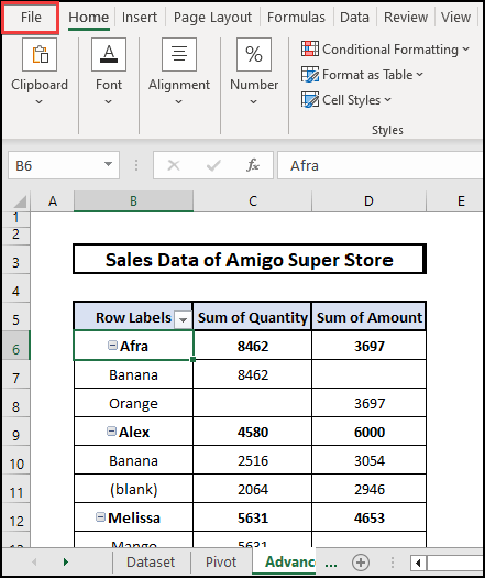
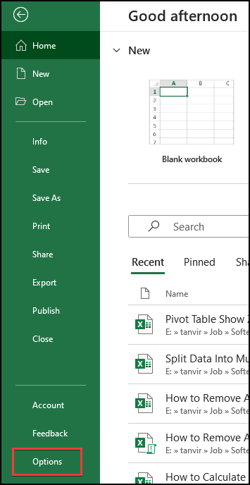
Primarily, click on the File menu from Top Ribbon.

Then, go to the Options feature.

Next, a box named Excel Options appears.
After that, go to the Advanced option and select the worksheet name in the Display Options for this Worksheet cell.
Further, select Show a zero in cells that have zero values to get zero in the blank cells.

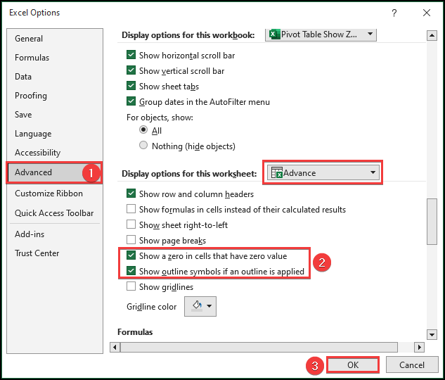
In the end, zero values are inserted in the blank cells of the pivot table.

method

3. Use VBA Macro to Input Zero Values

Using VBA code we can easily show zero in the pivot table in Excel. With the help of the Developer option, you can generate a program on your own. Please follow the necessary steps below.

⬇️⬇️ STEPS ⬇️⬇️

Check first if your Developer option is available or not.
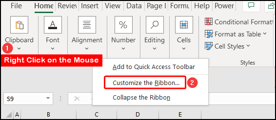
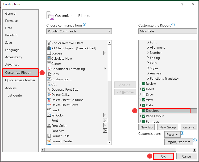
Secondly, to enable the Developer option, Right-Click on the mouse at the Top Ribbon and select Customize the Ribbon.

Thirdly, click on Developer and click on the OK button.

Now Developer mode is on.
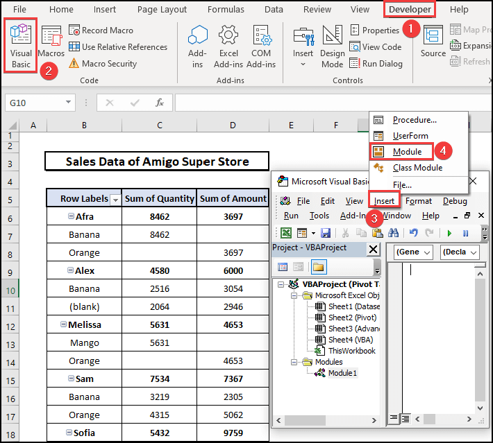
Then, click on the Visual Basic feature.
Next, to insert the VBA code, click on Module from the Insert menu.

Further, insert the following code and click on the Run icon.

Code

Sub VBA_1()
    Range("C6").Select
    ActiveSheet.PivotTables("PivotTable1").NullString = "0"
End Sub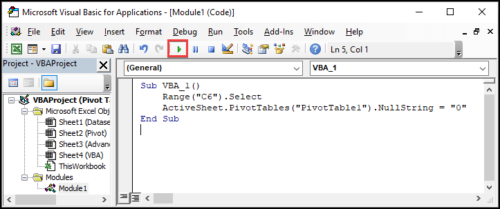

Finally, Zero was inserted in the blank cells.

method

4. Find Blanks and Insert Zero Values in Table

One of the easiest ways is to find the blanks and replace them with 0 in a dataset. Please follow the steps below.

⬇️⬇️ STEPS ⬇️⬇️

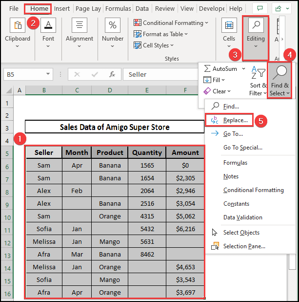
Initially, select the data range B5:F16.
Then drop down the Editing option from the Home menu of the Top Ribbon.
Next, navigate to the Find and Select option to select the Replace option.

Thus a box named Find and Replace appears.
Then, leave blank in the Find what cell and write 0 in the Replace with cell.
After that hit the Replace All button.

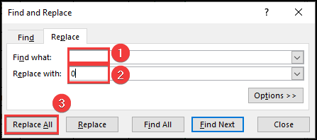
Therefore, automatically inserts 0 in 12 blank cells.

📄 Important Notes

🖊️ Enable the Developer menu first to execute VBA code.

🖊️ Keep in mind that the data type is not set to Accounting.

🖊️ Convert the dataset into Pivot Table first to get Pivot Table Options in the Context Menu list.

📝 Takeaway from This Article

📌 Pivot Table to filter and overview the dataset under criteria.

📌 Pivot Table Option to insert zero in the blank cells.

📌 Advance option from File of the Top Ribbon to keep the blank cells’ value 0 instead of blank.

📌 Find and Replace Feature to insert 0 in the blanks of the dataset.

📌 VBA to show zero in blank cells of Pivot Table.

Conclusion

We demonstrated every possible way to show zero values in Pivot Table in Excel. I hope you enjoyed your learning. Any suggestions, as well as queries, are appreciated. For better understanding and new knowledge, don’t forget to visit www.ExcelDen.com.

(Visited 37 times, 1 visits today)