Making a Pivot Table and measuring the weighted average in Excel is not everyone’s cup of tea. You can not simply modify or insert any formula in a pivot table to calculate the weighted average in Excel. Generally, we calculate the weighted average using SUMPRODUCT and SUM functions. On the contrary, we must follow alternative methods to calculate the weighted average. In this article, we will learn to measure and analyze the weighted average from a Pivot Table in Excel.
📁 Download Excel File
To practice please download the Excel file from here:
Learn to Measure Weighted Average from Pivot Table in Excel with These 3 Methods
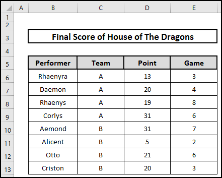
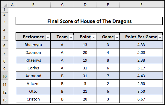
In this article, we are going to learn 3 catchy approaches to measure the weighted average from Pivot Table in Excel. Here we consider a dataset named Final Score of House of The Dragons containing Performer, Team, Point, and Game. There are 2 teams named Team A and B of 8 performers. To measure the weighted average we will explore the Pivot Table feature, the Table feature, and the use of an additional column. Later we will also learn the use of SUMPRODUCT and SUM functions to calculate the weighted average with percentages.
1. Analyzing Weighted Average with Pivot Table in Excel
Suppose you need to calculate the weighted average of points per game separately for both teams as well as an average of both teams. In this case, one can easily calculate and analyze the weighted average by converting a dataset into a Pivot Table. Please follow the steps below.
⬇️⬇️ STEPS ⬇️⬇️
- Initially, select the entire dataset B5:E13.
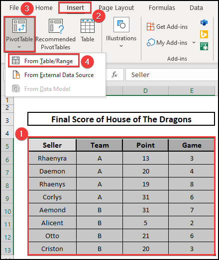
- Then, drop down the Pivot Table feature from the Insert menu.
- Next, select From table/Range option from the Pivot Table drop-down list.
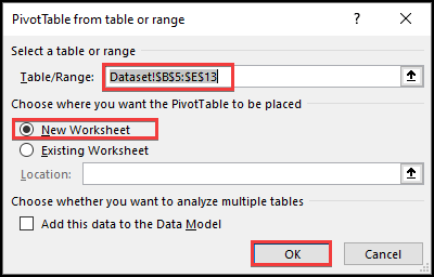
- Thus, a box named PivotTable from table or range appears.
- Next, type Dataset!$B$5:$E$13 in the Table/Range cell. Where range $B$5:$E$13 is mentioned from the Dataset sheet.
- Further, select New Worksheet to open and convert into Pivot Table into another sheet.
- Finally, hit the OK button.
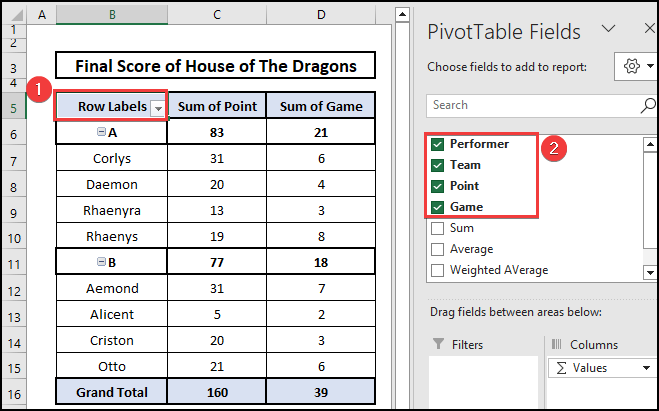
- In the meantime, Pivot Table appears in a new worksheet.
- In addition, select Performer, Team, Point, and Game options from the PivotTable Fields side ribbon to show in the Pivot Table.
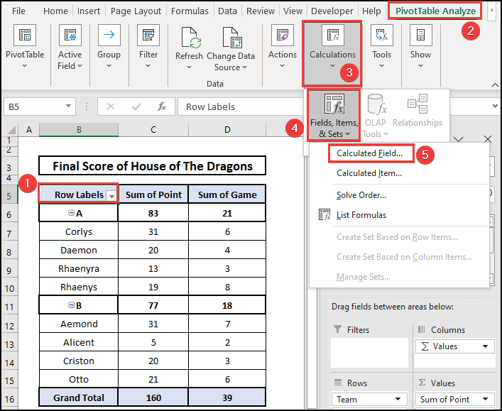
- Now, to calculate the weighted average we need to click on a cell i.e. B5 in the Pivot Table.
- Then go to the PivotTable Analyzer from the Top Ribbon.
- Next, navigate the Fields, Items & Sets feature from the Calculation segment.
- Further, select the Calculated Field option from the Fields, Items & Sets feature.
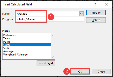
- Again another box named Insert Calculated Field appears.
- Now, insert Average in the Name field and {=Point/Game} in the Formula field.
- After that, hit the OK button to get new columns named Sum of Average.
- Therefore, a new column of data appears in column E named Sum of Average.
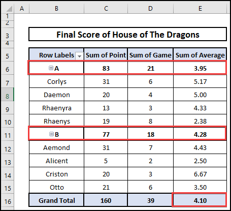
- In the E6 and E11 cells, the Average of teams A and B were observed respectively 3.95 and 4.28. Also, 4.10 is the average for teams A and B.
📕 Read More: 6 Quick Ways to Calculate Average Percentage of Marks in Excel
2. By Creating Excel Table
From converting the dataset into a Table, One can also calculate the weighted average without any hustle. Please follow the necessary steps.
⬇️⬇️ STEPS ⬇️⬇️
- First, select the entire dataset B5:E13.
- Secondly, click on the Table feature from the Insert menu of the Top Ribbon.
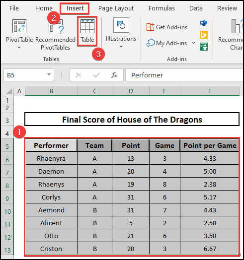
- Thirdly, the dataset converts into a table, and a drop-down box appears beside each heading.
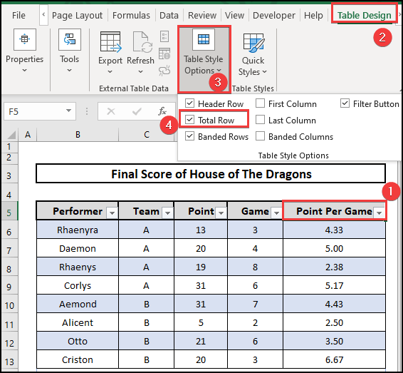
- Then go to the Table Design menu from the Top Ribbon and drop down the Table Style Option list.
- Next, click on Total Row from the Table Style Option lists.
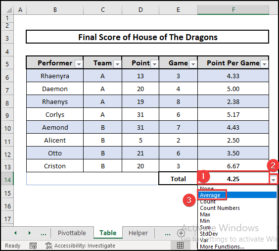
- Now click on cell F14. In addition, a drop-down box appears beside the cell.
- Then, navigate to the dropdown box list and click on the Average option from the list.
- Finally, the Average of F6:F13 delineated at the F14 = 4.25.
3. Using a Helper Column
With the help of an additional column, one can easily measure the weighted average in Excel easily. Please check out the below.
⬇️⬇️ STEPS ⬇️⬇️
- Primarily, select a blank cell i.e. B6.
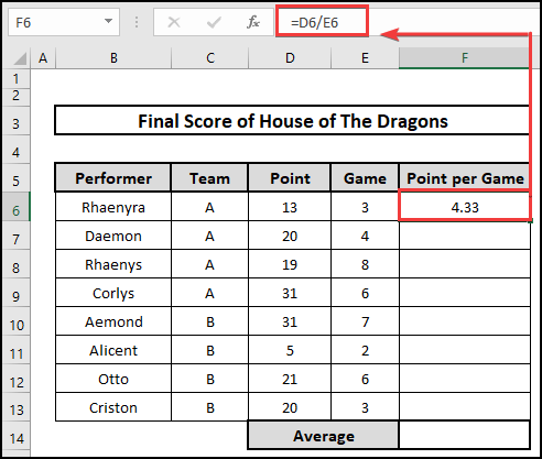
- Then, Divide the Point (D6) by Game (E6) to get the point per game.
=D6/E6
- Now, pull down the Fill Handle to fill the cells accordingly.
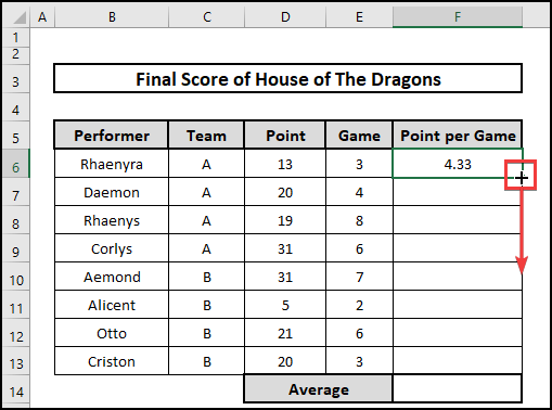
- Therefore, we get a point per game for each performer.
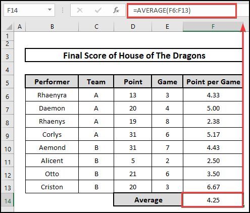
- Again, navigate cell F14 and insert the following formula to get the average of the F6:F13 range.
=Average(F6:F13)
- Finally, we obtain the weighted average of 4.25 in the F14 cell.
Calculate Weighted Average with Percentages Using SUMPRODUCT in Excel
If you have a dataset containing score and their weight in percentages. Now you are asked to calculate the weighted average. The use of the SUMPRODUCT function can be a key to calculating the weighted average. Please follow the procedure below.
⬇️⬇️ STEPS ⬇️⬇️
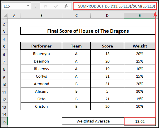
- Primarily, select a blank cell i.e. F15 to get the weighted average of percentages.
- Secondarily, insert the following formula in the F15 cell.
=SUMPRODUCT(D6:D13,E6:E13)/SUM(E6:E13)
- The SUMPRODUCT function multiplies between cells and sums up accordingly. Summing up the range E6:E13 divides the result of SUMPRODUCT function values.
- Therefore, we achieve the weighted average of 18.62 using the SUMPRODUCT function.
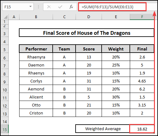
Calculate Weighted Average with Percentages in Excel
Again anyone can calculate the weighted average by multiplying the score and percentage. Then sum up the product and divide by the sum of the percentages. Please check out the below steps.
⬇️⬇️ STEPS ⬇️⬇️
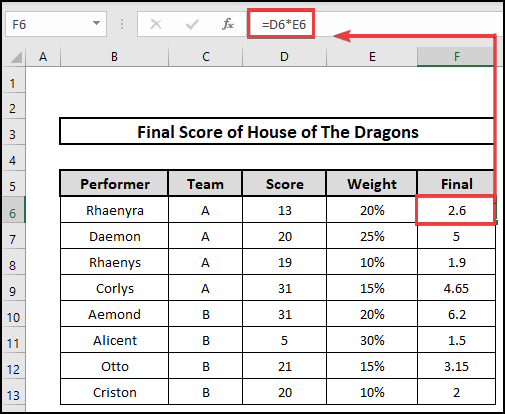
- Firstly, select a blank cell i.e. F15 to get the weighted average of percentages.
- Secondly, multiply D6 and E6 in the F6 cell and fill the cells automatically.
=D6*E6
- Therefore, we obtain the product for each cell.
- Now, select a blank cell i.e. F15 to get the weighted average of percentages.
- After that, insert the following formula in the F15 cell.
=SUM(F6:F13)/SUM(E6:E13)
- Sum of product F6:F13 divided by the sum of weight E6:E13.
- Therefore, we achieve a weighted average of 18.62 in the F15 cell.
📄 Important Notes
🖊️ Pivot Table doesn’t allow changes manually.
🖊️ Making a Table is important to get the average automatically from the dataset.
🖊️ Use of SUMPRODUCT and SUM functions leads to the same result.
📝 Takeaway from This Article
📌 Pivot Table to calculate weighted average in Excel.
📌 Table feature to measure average automatically.
📌 Helper column that supports measuring weighted average.
📌 SUMPRODUCT and SUM functions to measure weighted averages with percentages in Excel.
Conclusion
We demonstrated possible ways to calculate the weighted average using Pivot Table in Excel. I hope you enjoyed your learning. Any suggestions, as well as queries, are appreciated. Don’t forget to leave your thoughts in the comment section. For better understanding and new knowledge, don’t forget to visit www.ExcelDen.com.