Microsoft Excel is an integral element of our everyday routine. Excel is the program that first comes to mind when discussing data. Meanwhile, Excel is incredibly flexible and allows us to perform a wide range of data manipulations. When processing massive volumes of information, the SUMIFS function is indispensable. Accordingly, this article will describe how to use Excel’s SUMIFS function for multiple criteria in a Column and a Row. However, we start with a set of data that describes a company’s Products, Products, dates, and revenues.
📁 Download Excel File
You can download the practice workbook from here.
Overview of SUMIFS Function
If you employ the SUMIF function in Excel, the program tallies up all the results that match the criteria you set. The first three parameters are the range of cells to examine, the value to use as a condition, and the range from which to tally the results. There are therefore three arguments to set.
Syntax
SUMIF(range, criteria, [sum_range])
Arguments
- Range: A set of cells to search for criteria.
- Criteria: A criterion that can take the form of a number, text, expression, cell reference, or function.
- [Sum_Range]: A cell range containing the values to sum.
Learn to Use SUMIFS Function with Multiple Criteria Along Column and Row in Excel with 6 These Ways
For instance, six distinct SUMIFS-based approaches will be used in this article to calculate profit under multiple criteria in a row and a column. First, fill out the data set using criterion and result cells. Here, we take into account a Company data set. The columns of this data collection are labeled “Product,” “Continents,” “Date,” and “Revenue”. Likewise, we are going to use the SUMIFS function to calculate the sum under multiple criteria in a column and a row.
1. Using SUMIFS Function with Multiple Criteria
In this method, we will SUMIF function with multiple criteria for both in a single column and different columns to sum the required data. The examples are given below:
1.1 Criteria in Different Columns
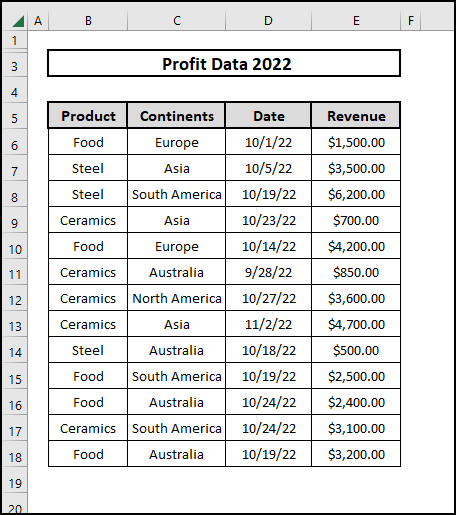
In this approach, we will use the SUMIFS function to estimate the sum of revenue for the selected Product (Ceramics) and Continent (Asia).
⬇️⬇️ STEPS ⬇️⬇️
- Firstly select cell H7.
- Then insert the SUMIFS.
- Write the following formula:
=SUMIFS(E6:E18,B6:B18,H5,C6:C18,H6)
- Finally, press Enter to see the results.
Thus, we have got the Total Revenue of the selected Continent and Product. Using a similar formula, you can calculate the sum with multiple criteria in the different columns.
🔨 Formula Breakdown
👉 Range = E6:E18: This is the Cell Range where the SUMIF function will be used.
👉 Criteria 1 = B6:B18,H5: Here, function will check which cells of range B6:B18 Match with cell value of H5.
👉 Criteria 2 = C6:C18,H6: This criterion says that cell values would be matched with cell value H6.
👉 Finally, the SUMIFS function will sum the cell values which will meet the given criteria in the selected cell range.
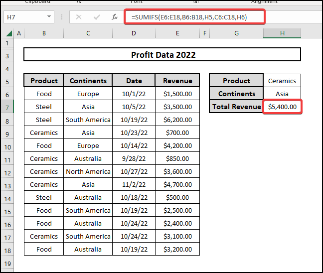
1.2 Criteria in the Same Column
In this method, we’ll utilize the SUMIFS function to calculate the Total Revenue for the Continent (Asia).
⬇️⬇️ STEPS ⬇️⬇️
- First, select cell H7.
- Second, insert the SUMIFS.
- Write the following formula:
=SUMIFS(E6:E18,C6:C18,H6)
- Lastly, press Enter to see the results.
As a result, we now have the Total Revenue for the chosen Continents and Products. You can calculate the sum with many criteria in the same column using a similar technique.
📕 Read More: SUMIFS with Multiple Criteria in Different Columns in Excel
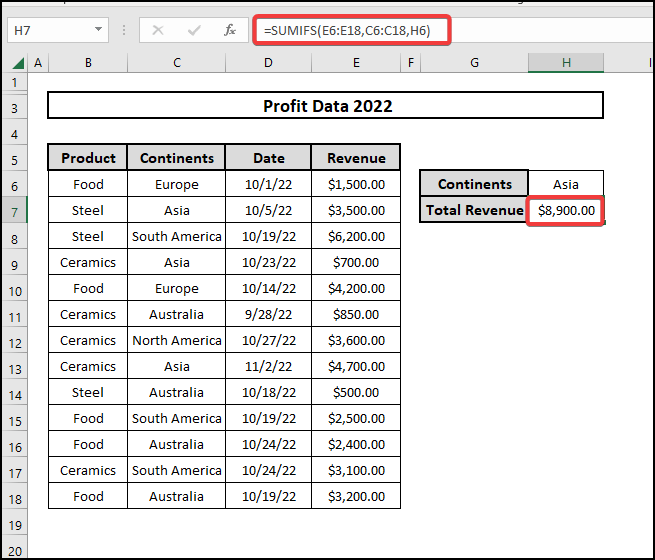
2. Using SUMIFS Function with Multiple Criteria and Comparison Operators Between Two Columns in Excel
What we’re looking for is a sum for Ceramics’ revenues that are under $3000 that can be derived from our data collection.
- Select the cell H7.
- Insert SUMIFS function consequently.
- Write the following formula:
=SUMIFS(E6:E18,B6:B18,H5,E6:E18,”>”&H6)
- Then press Enter to see the results.
🔨 Formula Breakdown
👉 Range = E6:E18: This is the Cell Range where the SUMIF function will be used.
👉 Criteria 1 = D6:D18,”>”&H5: Here, the function will check which cells of range D6:D18 are greater than the cell value of H5.
👉 Criteria 2 = D6:D18,”<“&H6: seconnd criteria is to check which cells of range D6:D18 are greater than H6.
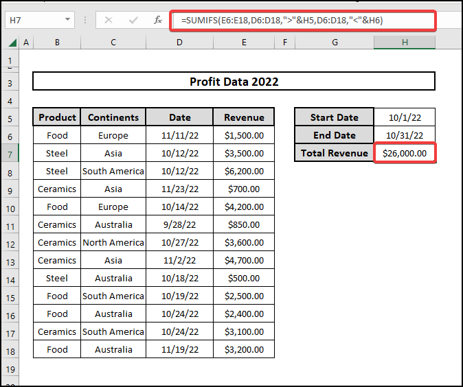
3. Using SUMIFS Function Containing Date Criteria Along Column
Find out how revenues stack up to this point in time. Let’s figure out October’s sales numbers. By using the SUMIFS function.
⬇️⬇️ STEPS ⬇️⬇️
- Firstly, select cell H7.
- Next, insert the SUMIFS function.
- Consequently, write the formula:
=SUMIFS(E6:E18,D6:D18,”>”&H5,D6:D18,”<“&H6)
- At last, hit Enter to see the results.
- As a result, we have the total income for the indicated Product or Continents. The same procedure can compute totals based on several criteria in the same column.
🔨 Formula Breakdown
👉 Range = E6:E18: This is the selected Cell Range where the SUMIF function will operate.
👉 Criteria 1 = D6:D18,”>”&H5: Here, function will check which cells of range D6:D18 are greater than the cell value of H5.
👉 Criteria 2 = D6:D18,”<“&H6. Here, the function denotes cells of range D6:D18 are less than the cell value H6.
📕 Read More: 7 Examples to Use SUMIFS with Multiple Criteria in Same Column
4. Using SUMIFS Function for Blank Rows
Delete two entries from the dataset to create a sheet containing blank cells. Now we will estimate the revenue from the rows that contain blank cells.
⬇️⬇️ STEPS ⬇️⬇️
- Select cell H6.
- Insert SUMIFS function.
- Insert the formula below:
=SUMIFS(E6:E18,B6:B18,””,C6:C18,””)
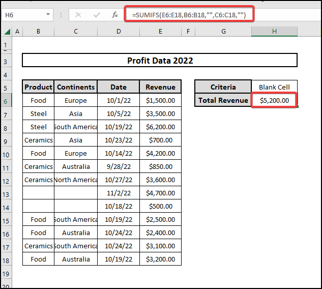
- Then press Enter to see the results.
Consequently, we have the entire income for the given Product or Continent. Using the same procedure, totals based on various criteria in the same column can be calculated.
🔨 Formula Breakdown
👉 Range = E6:E18:This is the cell range that will be used by the SUMIF function when it is applied.
👉 Criteria 1 = B6:B18,””,C6:C18,”” : In this part, the function will examine the blank cells of the range. D6:D18.
👉 Criteria 2 = C6:C18,””: Here, the function will check empty cells of range C6:C18.
5. Using SUMIFS Function for Non-Blank Cells in Both Column and Row
In this case, we’ll use two formulas. SUMIFs with SUM function first and only SUMIFS later to calculate the total Revenue of nonblank cells.
5.1 SUM with SUMIFS Functions
We will use the SUM function to total Revenue and SUMIFS to sum blank cell revenue. Then subtraction will be carried out.
⬇️⬇️ STEPS ⬇️⬇️
- First, Select cell H6.
- Consequently, write down the following formula:
=SUM(E6:E18)-SUMIFS(E6:E18,B6:B18,””,C6:C18,””)
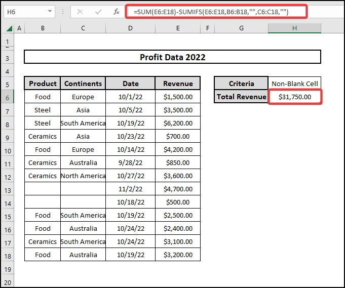
- Hit Enter to view the results.
Total income for the selected Product or Continents. Multiple columns can be totaled using the same procedure.
🔨 Formula Breakdown
👉 Range = E6:E18:This is the Cell Range where the SUMIF function will operate.
👉 Criteria 1 = B6:B18,””,C6:C18,”” : Here, the function will check blank cells of range D6:D18.
👉 Criteria 2 = C6:C18,””: Here, the function will check empty cells of range C6:C18.
5.2 SUMIFS Function Only
Just employing the SUMIFS function can we determine the sum of all cells that are not blank in particular.
⬇️⬇️ STEPS ⬇️⬇️
- Pick cell H6.
- Insert the following formula:
=SUMIFS(E6:E18,B6:B18,”<>”,C6:C18,”<>”)
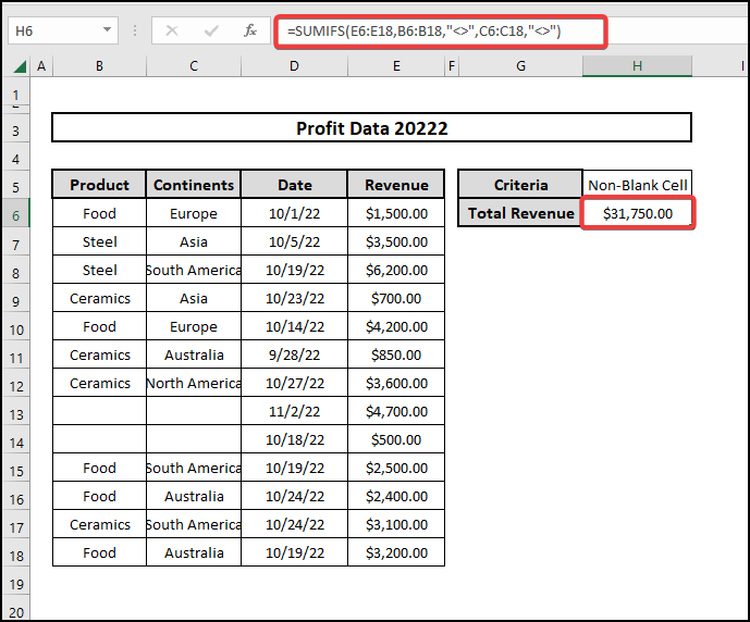
- Hit Enter to see the results.
As a result, we have a total product or continent income. So, Totals based on various criteria in the same column can be computed using the same procedure.
🔨 Formula Breakdown
👉 Range = E6:E18: This is the selected Cell Range where the SUMIF function will work.
👉 Range = E6:E18:Here is the range of cells where the SUMIF function will be utilized.
👉 Criteria 1 = B6:B18,”<>”,C6:C18,”<>” : Here, the function will check nonblank cells of range D6:D18.
👉 Criteria 2 = C6:C18,””: Here, the function will check non-blank cells of range C6:C18.
6. Using SUMIFS Function with Multiple OR Criteria in Excel
We will try to solve this by using the SUMIFS function first and the array argument with the SUMIF function in this method later.
6.1 Using SUMIFS Function Only
Let’s apply the SUMIFS function with multiple OR criteria first.
⬇️⬇️ STEPS ⬇️⬇️
- Pick cell H9.
- Write down the following formula:
=SUMIFS(E6:E18,D6:D18,”>”&H5,D6:D18,”<“&H6,C6:C18,H7)+SUMIFS(E6:E18,D6:D18,”>”&H5,D6:D18,”<“&H6,C6:C18,H8)
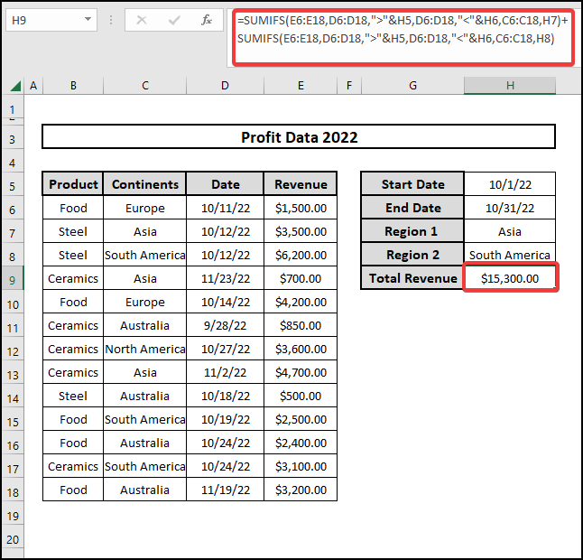
- Then hit Enter to see the results.
🔨 Formula Breakdown
👉 SUMIFS functions to sum all the data under the applied criteria
👉 Range = E6:E18: This is the selected Cell Range where the SUMIF function will work.
👉 Criteria 1 = D6:D18,”>”&H5: Here, function will check which cells of range D6:D18 are greater than the cell value of H5.
👉 Criteria 2 = D6:D18,”<“&H6. Here, the function denotes cells of range D6:D18 are less than the cell value H6.
👉 Criteria 3 = C6:C18,H7. Here, the function means cells of range C6:C18 contain the H7 value.
👉 The second part of the formula also follows the same.
6.2 Using Array Argument in SUMIF Function
We will use the combination of SUM and SUMIF functions to calculate the Revenue for Asia and Europe region.
⬇️⬇️ STEPS ⬇️⬇️
- Pick cell H7.
- Write down the following formula:
=SUM(SUMIF(C6:C18,{“Asia”,”Europe”},E6:E18))
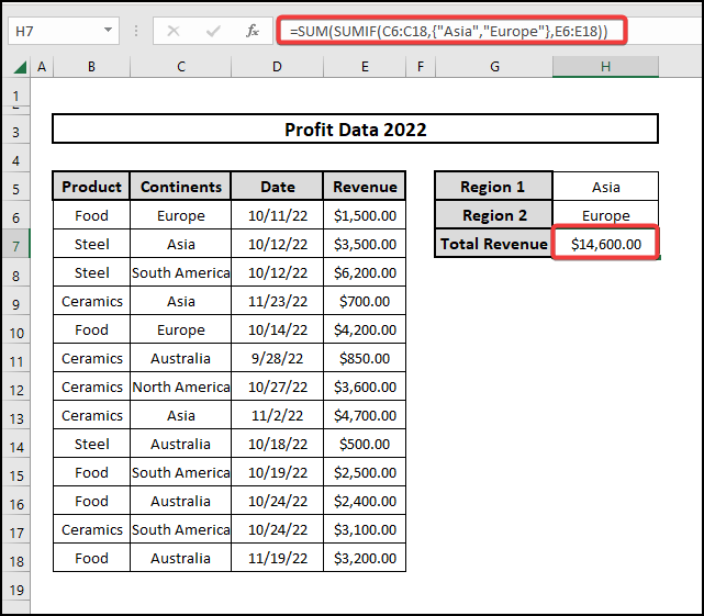
- Then hit Enter to see the results.
🔨 Formula Breakdown
👉 SUM functions sum all the data in the selected range.
👉 SUMIFS functions sum all the data under the applied criteria.
👉 Range = C6:C18: This is the selected Cell Range where the SUMIF function will work.
👉 Criteria = {“Asia”,”Europe”}: Here, the function will check the value containing “Asia” and “Europe”.
👉 Range = E6:E18: the function will operate on the specified range of cells.
📄 Important Notes
🖊️ Verify that you’ve selected the criteria when it was required.
🖊️ Also, always look for ways that are easy to use in different situations.
🖊️ In addition, every time try to use shortcuts on the keyboard.
📝 Takeaways from This Article
📌 Firstly, you can calculate total profit under different criteria by applying the SUMIFS function
📌 Also, you can use the SUMIFS function in different circumstances.
Conclusion
In particular, we demonstrated some applications of the SUMIFS function for multiple criteria in a Column and a row. Moreover, We’ve included several alternatives to SUMIFS as well. Expect this is the precise answer you’ve been seeking. Join us and share your thoughts. So, please use the comment section below to ask any queries or make any comments. Eventually, Visit ExcelDen.com to look through more articles about Excel.


