The SUMIFS Function is useful in ways that it can add up numbers using multiple criteria. We can use SUMIFS with multiple criteria in the same column in Excel by various approaches. In this article, we will be talking about 7 such different approaches to using SUMIFS with multiple criteria in the same column.
📁 Download Excel File
Download the practice workbook below.
Overview of SUMIFS Function
The SUMIFS Function is defined as follows:
SUMIFS(sum_range, criteria_range1, criteria1, [criteria_range2, criteria2], ...)Where, Sum_range (required)= The range of cell to sum.
Criteria_range1 (required)= the initial range to be assessed against the relevant criteria. (Required).
Criteria1 (required)= The initial condition that must be met.
Criteria_range2, criteria2, …(optional)= Extra ranges and criteria associated. (Optional).
Learn to Use SUMIFS with Multiple Criteria in Same Column in Excel with These 7 Examples
To illustrate things clearly, let us consider a dataset of different products, their types, price, and their order date. Using this dataset, we will now be looking at 7 approaches to using the SUMIFS Function with multiple criteria in the same column in Excel. The approaches are discussed as follows:

1. Using SUMIFS for OR Logic
We can use the SUM and SUMIFS Functions and OR logic to find different results. In this dataset, we will be using the function to find the total price of phones and tablets. Here are the steps for the processes.
⬇️⬇️ STEPS ⬇️⬇️
- First, we select cell D14.
- We write the following formula down in the formula bar and press Enter.
=SUM(SUMIFS(E6:E11,D6:D11,{"Phone","Tablet"}))
- The Total Price of Phones and Tablets will be visible in the following image as the output or the result:

📕 Read More: SUMIFS with Multiple Criteria in Different Columns in Excel
2. Utilizing SUMIFS for OR Logic with Wildcards
This approach is quite similar to that of the previous one. However, in this method, instead of giving the total string of text to the SUMIFS Function, we insert words beginning with a * sign to match the exact word in the dataset. The steps are as follows:
⬇️⬇️ STEPS ⬇️⬇️
- First, we select cell D14.
- We write the following formula down in the formula bar and press Enter.
=SUM(SUMIFS(E6:E11,D6:D11,{"*Phone","*Tablet"}))
- The Total Price of Phones and Tablets will be visible in the following image as the output or the result:

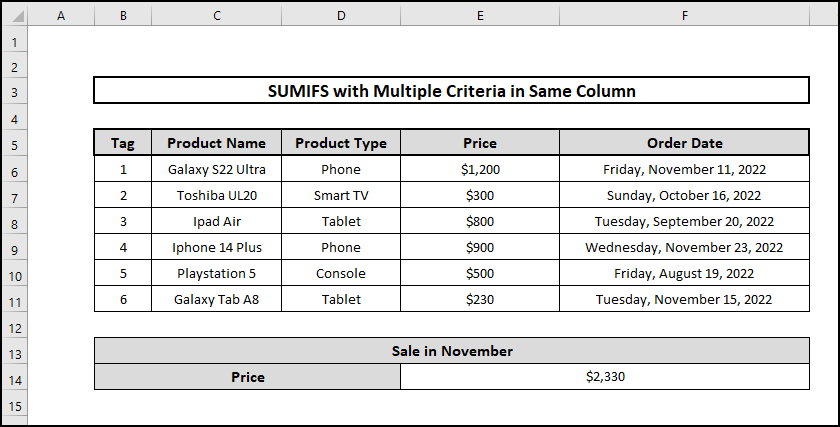
3. Applying SUMIFS with Dates
In this method, we will be using the SUMIFS function with multiple criteria in the same column for date format. Suppose we have the order dates for the products and we want to find out the total sale of products in the last 30 days in the month of November. The steps for this process are as follows:
⬇️⬇️ STEPS ⬇️⬇️
- Firstly, we select cell E14.
- Then we write the following formula in the formula bar:
=SUMIFS(E6:E11, F6:F11,">="&TODAY()-30, F6:F11,"<="&TODAY())🔨 Formula Breakdown
SUMIFS(E6:E11, F6:F11,”>=”&TODAY()-30, F6:F11,”<=”&TODAY())
👉 The TODAY Function returns the serial number of the current date. This Function hence changes the cell format to Date after its application to a cell.
👉 This Function syntax does not have any arguments.
👉 In the above formula, we give the range of the cell as E6:E11 and the conditional range as F6:F11.
👉 Then we see if the criteria range is within the last 30 days from today. So, if it is 27th of November today, this Function will filter and sum data later than the 27th of October.

- Now we press Enter.
- We will see the results as output like the following image:
4. Using SUMIFS with Comparison Operators
Suppose we want to find out the price of phones above 500 dollars and sum the worth of the phones. In this example, we will be using the comparison operator >= in the SUMIFS Function to find out the results. The steps for this process are as follows:
⬇️⬇️ STEPS ⬇️⬇️
- First, we select cell E13.
- Then we write the following formula in the formula bar:
=SUMIFS(E6:E11,D6:D11,"Phone",E6:E11,">=500")🔨 Formula Breakdown
SUMIFS(E6:E11,D6:D11,”Phone”,E6:E11,”>=500″)
👉 Here E6:E11 denote sum range, D6:D11 indicate criteria range.
👉 “Phone” is the criteria and >= is the comparison operator that is indicating to take phone prices greater than or equal to 500.

- After that, we press Enter. The table of results will be like the image below:

5. Implementing SUMIFS Function with Blank and Non-Blank Cells
Often in large spreadsheets, we have to sum blank and non-blank cells. On this occasion, we will be looking at an example that will make us understand how to use the SUMIFS function to sum blank and non-blank cells. The steps are as follows:
⬇️⬇️ STEPS ⬇️⬇️
- First, we select cell F13.
- After that, we input the following formula in the formula bar and press Enter.
=SUMIFS(E6:E11, F6:F11,"<>", G6:G11,"=")🔨 Formula Breakdown
SUMIFS(E6:E11, F6:F11,”<>”, G6:G11,”=”)
Here in the SUMIFS Function,
👉 E6:E11 evidently indicates the sum range
👉 F6:F11 and G6:G11 denote the criteria range.
👉 F6:F11 is followed by a “<>” sign which means to sum values of cells that are non-empty
👉 G6:G11 is followed by a “=” sign that indicates to sum values corresponding to blank cells.
This means, indeed, that the formula will identify the cells that are blank in the delivered date column and add their prices.

- We will see that the output will take multiple criteria and only give the sum where the product delivery date is missing, that is the price of the non-delivered products. The results are shown as follows:

6. Using SUMIFS Function Multiple OR Criteria
In this method, we use comparison operators to select the range of dates and also use the multiple SUMIFS functions. For the particular dataset, this method is explained as follows:
⬇️⬇️ STEPS ⬇️⬇️
- We select cell J8.
- Then, we write the following formula down.
=SUMIFS(G6:G11,D6:D11,J6,F6:F11,">=11/1/2022",F6:F11,"<=11/30/2022")+SUMIFS(G6:G11,D6:D11,J7,F6:F11,">=11/1/2022",F6:F11,"<=11/30/2022")🔨 Formula Breakdown
SUMIFS(G6:G11,D6:D11,J6,F6:F11,”>=11/1/2022″,F6:F11,”<=11/30/2022″)+SUMIFS(G6:G11,D6:D11,J7,F6:F11,”>=11/1/2022″,F6:F11,”<=11/30/2022″)
We used 2 SUMIF Functions for two brands Apple and Samsung. In the formula SUMIFS(G6:G11,D6:D11,J6,F6:F11,”>=11/1/2022″,F6:F11,”<=11/30/2022″),
👉 G6:G11 specifies the sum range
👉 D6:D11 represents the criteria range where the criterion we’re choosing is called Apple and we have specified it in cell J6.
👉 The range of cells F6:F11 indicates the order date and the logic after that indicates to pick values from 11.1.2022 to 11.30.2022.
👉 Consequently, for the other SUMIF Function, everything will be the same except now we’ll do the same for Samsung indicated in cell J7.

- After that, we press Enter.
- Thus, we will get the total price of products of Apple and Samsung in the month of November as follows:

📕 Read More: Use SUMIFS for Multiple Criteria in Column and Row in Excel
7. Applying SUMIFS Function Multiple OR Criteria in One Column
Now, we will be applying SUMIFS Function with multiple criteria in the same column. That is, we will be using separate SUMIF Functions and adding them up. For the first SUMIF Function, the product type will be phone and the second product type will be consoled. The steps for this process are as follows:
⬇️⬇️ STEPS ⬇️⬇️
- First, we specify the cells G5 and G6 by writing the names of product types as Phone and Console.
- Now we select cell G7 and incorporate the following formula.
=SUMIF(C6:C11,G5,D6:D11) + SUMIF(C6:C11,G6,D6:D11)🔨 Formula Breakdown
SUMIF(C6:C11,G5,D6:D11) + SUMIF(C6:C11,G6,D6:D11)
👉 Here, we have used two SUMIF Functions.
👉 The first SUMIF Function =SUMIF(C6:C11,G5,D6:D11) filters the product type Phone from the data and sums their prices.
👉 Similarly, the second SUMIF Function SUMIF(C6:C11,G6,D6:D11) filters the product type Console from the list and sums their prices.
👉 Finally, we add the two SUMIF Functions to get the total price of phones and consoles.

- Next, we press Enter.
- Now the total prices of phones and consoles will look like the following table:

📄 Important Notes
🖊️ We should take care while specifying the sum range, criteria range, and criteria inside the SUMIFS Function.
🖊️ In addition, we should also be careful with the comparison operators in different approaches as the results will come out different or not at all if there is any slight mistakes in such operators.
📝 Takeaways from This Article
You have taken the following summed-up inputs from the article:
📌 To sum up, we can use SUMIFS Function with OR logic, OR logic with wildcards or multiple OR logic to filter different criteria from a large dataset and find the sum of those cells that satisfy the criteria.
📌 Furthermore, we can use comparison operators to filter criteria and find their sum as well. We can also use SUMIFS Function with the TODAY Function to filter dates of events.
📌 We can also use SUMIFS Function with multiple criteria for blank and non-blank cells.
Conclusion
On the whole, this article will hopefully give you some insights about using the SUMIFS Function with multiple criteria in the same column. Besides, feel free to ask any questions related to the article in the comment section if you have any queries. If you want to know more, then follow ExcelDen for more Excel-related articles and solutions.


