Sometimes we need to find out, highlight or eradicate duplication in the same sheet. If duplications are in the same worksheet it is easier to eliminate or mark them. However, finding out duplication in the different sheets is not everyone’s mug of tea. Not only to eliminate duplication but also to match data among different sheets we need to learn the necessary approaches. Suppose we need to match this year’s best-seller ranking of the town to the previous year’s. In this case, comparison among data sheets may be essential to the judges and audience. In this article, we will learn the formula to compare two cells in different Excel Sheets.
📁 Download Excel File
To practice please download the Excel file from here:
Learn to Compare Two Cells in Different Sheets Using Formula in Excel with These 6 Methods
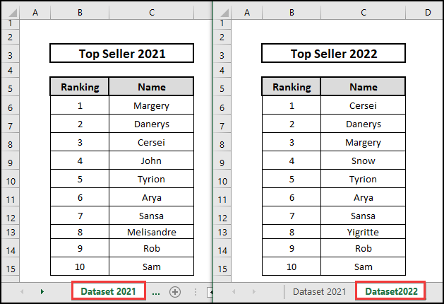
In this article, we expound 6 catchy approaches to compare two cells in different sheets using the formula in Excel. To construct the methods, we consider two datasets named Top Seller 2021 and Top Seller 2022 containing the Ranking and Name of the seller. There are also 3 columns along with 15 rows. We will learn Logical Expression as well as EXACT, IF, and VLOOKUP functions. The use of Conditional Formatting and VBA Macro will also be illustrated. So let’s get started.
1. Compare Two Excel Sheets for Differences in Values Using Logic
Comparing the cells of the Top seller of 2022 to the respective cells of the Top seller of 2021, one can quickly find out the similarity. Please check out the following procedure.
⬇️⬇️ STEPS ⬇️⬇️
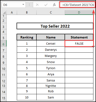
- Firstly, select a blank i.e. D6 under Statement heading.
- Secondly, input the following formula containing the logical expression.
=C6=’Dataset 2021′!C6
🔨 Formula Breakdown 👉 C6 look for the match in C6 of Dataset 2021 worksheet. 👉 If C6 is able to find a matching then it writes TRUE, else writes FALSE.
- Therefore by pressing Enter we get the result FALSE in the D6 cell which is the mismatched result to Dataset 2021 sheet.
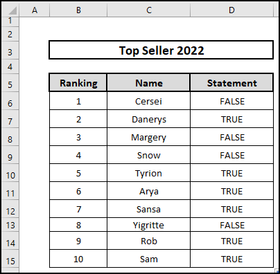
- Finally, by auto-filling the cells under the Statement heading, we obtain the result as TRUE or FALSE comparing two cells in different worksheets.
📕 Read More: 6 Easy Methods to Compare Two Strings in Excel for Similarity
2. Implement EXACT Formula to Compare Two cells in Different Sheets in Excel
Using the EXACT function one can extract similar cells based on True/False statements within a moment. The EXACT function is also a case-sensitive function. Syntax of EXACT function,
=EXACT(Value1,Value2)
⬇️⬇️ STEPS ⬇️⬇️
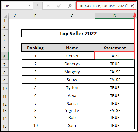
- Initially, select a cell i.e. D6 to get the result based on True-False under the Statement heading.
- Secondly, write the following formula in the D6 cell containing the EXACT function.
=EXACT(C6,’Dataset 2021′!C6)
🔨 Formula Breakdown 👉 EXACT function generally looks for the exactly matched value in the worksheet. 👉 Here, C6 of Dataset 2022 looks for the exact value in C6 of Dataset 2021 worksheet. 👉 Once, C6 finds out the exact match it delivers TRUE, otherwise it writes FALSE.
- Therefore by pressing Enter we get the result in the D6 cell comparing the Top seller of 2022 to the Top Seller of 2021.
- In the end, by auto-filling the cells under the Statement heading, we obtain the result as True or False comparing two cells in different worksheets.
📕 Read More: 5 Steps to Do Statistical Comparison of Two Data Sets in Excel
3. Apply IF Function to Compare Two Cells in Excel
IF function is a logical function that works based on True or False logic. Based on a logical test result, if two cells are similar then it can be written as Match, Else we can write Mismatch in an additional column. Syntax of IF function,
⬇️⬇️ STEPS ⬇️⬇️
- Primarily, select a blank i.e. D6 cell to get the result under the Statement heading.
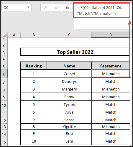
- Then, write the following formula in the D6 cell including the IF function.
=IF(C6=’Dataset 2021′!C6, “Match”,”Mismatch”)
🔨 Formula Breakdown 👉 Firstly, the IF function judge on a logical test. 👉 Secondly, If the logic is True then it writes Match in cell D6; Otherwise, Mismatch takes place in D6.
- Therefore by pressing Enter we get the result in the D6 cell.
- Lastly, by auto-filling the cells under the Statement heading, we obtain the result as Match or Mismatch comparing two cells in different worksheets.
4. Use VLOOKUP and ISNA Functions Combined
VLOOKUP function along with IF and ISNA functions can be a way to ferret out Matched names of Top Seller 2022 to Top seller 2021. VLOOKUP function generally finds the value in a selected range. The general syntax of the VLOOKUP function,
On the other hand, the IF function is a logical function that works based on True or False logic. Syntax of IF function,
Further ISNA function detects the N/A values. If it finds N/A, it will write True, else False. Syntax of ISNA function,
⬇️⬇️ STEPS ⬇️⬇️
- Firstly, select a blank i.e. D6 cell to get under the statement heading.
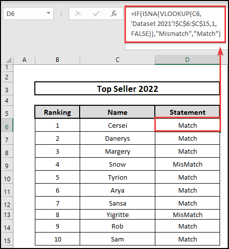
- Secondly, write the following formula in the D6 cell including IF, ISNA, and VLOOKUP functions.
=IF(ISNA(VLOOKUP(C6,’Dataset 2021′!$C$6:$C$15,1,FALSE)),”Mismatch”,”Match”)
🔨 Formula Breakdown 👉 Firstly, VLOOKUP(C6,’Dataset 2021′!$C$6:$C$15,1,FALSE); VLOOKUP function looks for the value of C6 in $C$6:$C$15 range of Dataset 2021 with a return value. 👉 Then, the ISNA function only deals with NA errors or texts. 👉 Finally, if the VLOOKUP function finds the value in the selected range, the IF function makes the statement based on availability. If it is unable to match then writes Mismatch; Else it writes Match in the D6 cell.
- Therefore by pressing enter we achieve the result in the D6 cell.
- Lastly, by auto-filling the cells of the Statement column, we obtain the result as a match or Mismatch.
- One thing, keep in mind the VLOOKUP function looks up values in the selected range. It doesn’t matter if it is in the same position or not. Rather it finds the value in the selected range dataset.
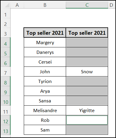
5. Use Conditional Formatting Feature
Using the Conditional Formatting feature, you can compare two cells in different sheets and highlight names with a color. Please follow the necessary steps below.
⬇️⬇️ STEPS ⬇️⬇️
- First, select the C6:C15 range.
- Then select New Rule from the Conditional Formatting feature of the Home tab.
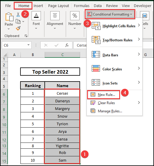
- Next, a box named New Formatting Rule appears.
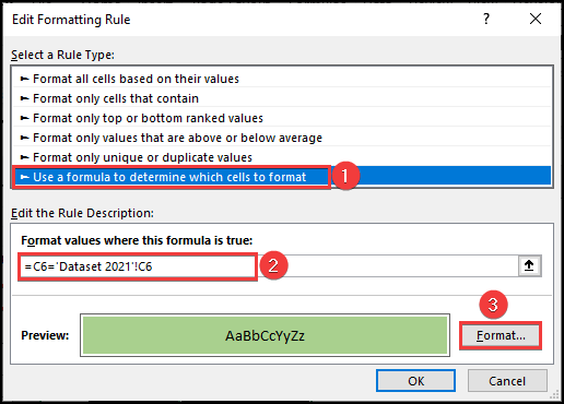
- After that, select Use a Formula to Determine Which Cells to Format from the Select a Rule Type section.
- Further, write =C6=’Dataset 2021’!C6 in the Format values where this formula is true cell.
- Also, click on the Format button to change color and observe from the preview box.
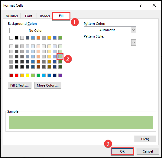
- Thus, another cell named Format Cells appears.
- Afterward, select the color and hit the OK button from the Fill menu,
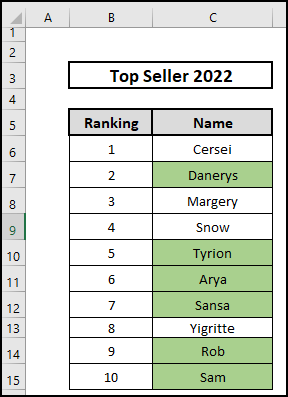
- Therefore, all the cells containing names get colored that are to the Top Seller 2021.
6. Utilize Excel VBA Macro
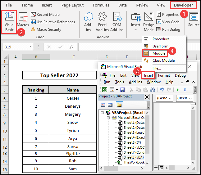
Generating a VBA code, one can compare two cells in different sheets without demur. By getting the Developer option in the Top Ribbon, you can generate a program on your own. Please follow the necessary steps below.
⬇️⬇️ STEPS ⬇️⬇️
- Check first if your Developer option is available or not.
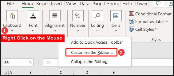
- Secondly, to enable the Developer option, Right-Click on the mouse at the Top Ribbon and select Customize the Ribbon.
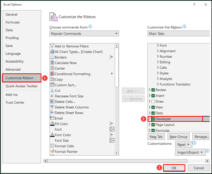
- Thirdly, click on the Developer option and hit the OK button.
- Now Developer mode is on.
- Then, click on the Visual Basic feature.
- Next, to insert the VBA code, click on Module from the Insert menu.
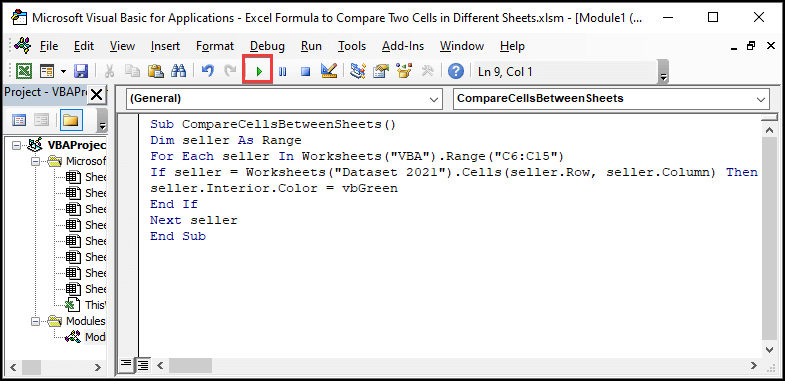
- Now, input the following code in the VBA module of the Worksheet.
- After that, select the dataset range C6:C15 and click on the Run icon.
Code
Sub Compare_Two_Cells_in_Different_Sheets()
Dim seller As Range
For Each seller In Worksheets("VBA").Range("C6:C15")
If seller = Worksheets("Dataset 2021").Cells(seller.Row, seller.Column) Then
seller.Interior.Color = vbGreen
End If
Next seller
End Sub
🔨 Formula Breakdown
👉 Firstly, declare seller in the range.
👉 Secondly, dictate that the seller is situated in the C6:C15 range of VBA worksheet.
👉 Thirdly, compare each seller to the Dataset 2021 worksheet.
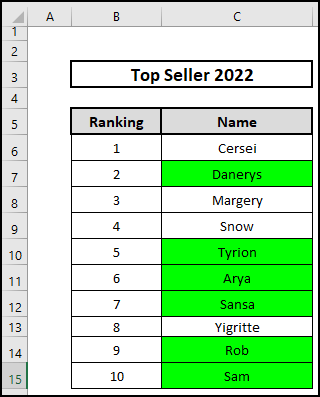
👉 Finally, If names are found in Dataset 2021 worksheet, Then make the cell color Green.
- Finally, we obtain the Top Seller of 2022 that is matched to 2021 and highlighted with Green color.
How to Compare Two Columns and Count Matches in Excel
Selecting the data range and Using SUMPRODUCT and SUM functions one can count matches as well as mismatches without demur. Please check out the necessary steps below.
⬇️⬇️ STEPS ⬇️⬇️
- First, select a blank i.e. F6 cell to get Match numbers from the dataset.
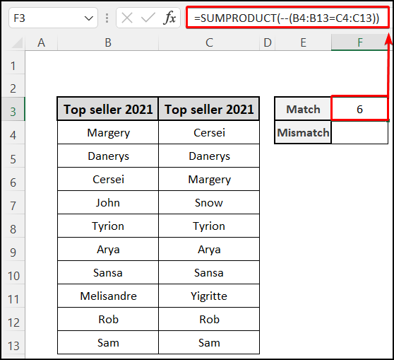
- Second, type the following formula in the F3 cell containing the SUMPRODUCT function.
=SUMPRODUCT(–(B4:B13=C4:C13))
- Here, B4:B13 range matches to the range C4:C13. In contrast, the SUMPRODUCT function counts the matches.
- Therefore, obtain the 6 matches from the data of two columns.
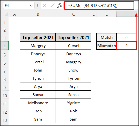
- Again, use the following formula containing the SUM function in the F4 cell to get the mismatched names.
=SUM(–(B4:B13<>C4:C13))
- Here, B4:B13<>C4:C13 means finds the dissimilar names from this two range.
- Finally, like matched value, obtain 4 mismatched names in the F4 cell.
How to Compare Two Columns and Remove Duplicates in Excel
The Conditional Formatting feature is an essential feature to Compare two columns and sort out duplicates with box color. Marking with a suitable color and deleting them, you can eradicate duplicates quickly. Please check out the steps below.
⬇️⬇️ STEPS ⬇️⬇️
- First, select the B4:C13 range.
- Then select New Rule from the Conditional Formatting feature of the Home tab.
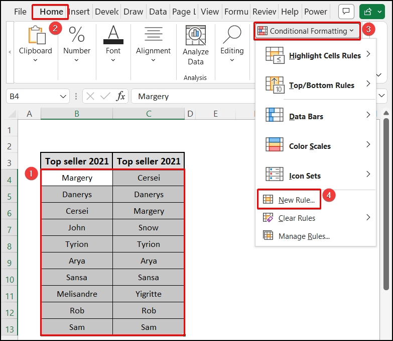
- Next, a box named New Formatting Rule appears.
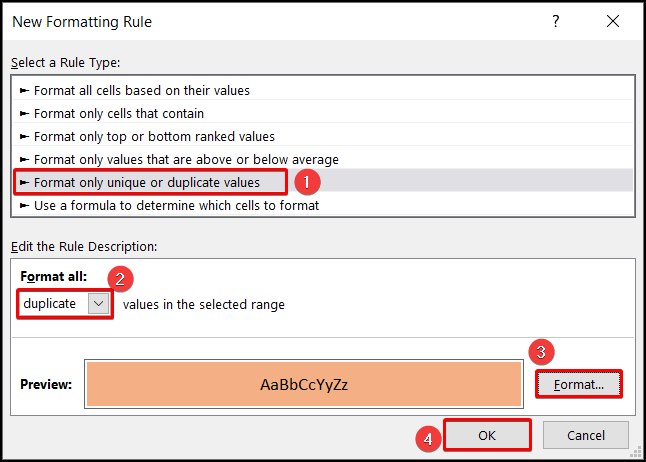
- After that, select Format Only Unique or Duplicate Values to Format from the Select a Rule Type section.
- Further select Duplicate from the drop-down box in the Format all option.
- Afterward, click on the Format button to change color and observe the color from the preview box.
- Finally, hit the OK button to proceed.
- Therefore, we obtain the colored cells that contain duplication.
- After that, select the duplicate cells from column C and press Delete to erase them.
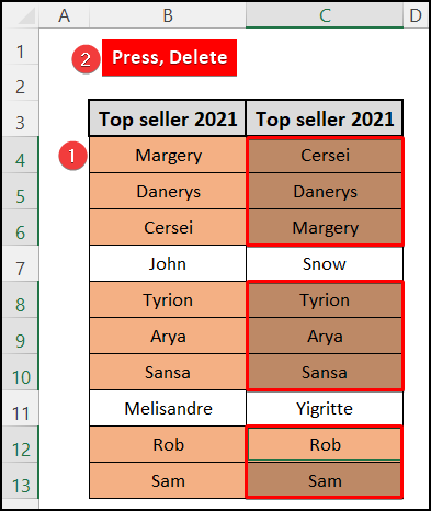
- In the end, removing the duplicate cells from column C, now we obtain the unique values in two columns.
📄 Important Notes
🖊️ Enable the Developer menu first to execute VBA code.
🖊️ ISNA function only deals with N/A value or error.
🖊️ EXACT function is a cases-sensitive function. The function has issues with lower-cases and higher-cases dissimilarity.
🖊️ VLOOKUP function looks for its value in the selected range. However, it doesn’t consider the value of a cell to cell.
📝 Takeaways from This Article
📌 General logical expression to compare two cells in different worksheets.
📌 EXACT function to match the values exactly.
📌 IF function for logical tests and make a statement based on them.
📌 ISNA function to find out N/A in cells.
📌 VLOOKUP function to look up a value in the selected range.
📌 Conditional Formatting feature to compare, find out duplications and highlight with color.
📌 VBA Macro to compare between different sheets and highlight the cells.
📌 SUMPRODUCT and SUM functions to count Match and Mismatch cells.
Conclusion
In this article, we construe 6 approaches to compare two cells using formulas in different sheets in Excel. I hope you enjoyed your learning and will be able to compare and highlight the cells based on values. Any suggestions, as well as queries, are appreciated. Don’t hesitate to leave your thoughts in the comment section. For better understanding and new knowledge, don’t forget to visit www.ExcelDen.com.


