In this article, I’ll show you three excellent methods on how to apply formula to change text color based on value in Excel. Furthermore, these strategies will allow you to solve the problem that brought you here. However, you will learn some important Excel features and functions in this post that will come in handy for any Excel job.
📁 Download Excel File
Download your free workbook from here.
Learn to Apply Excel Formula to Change Text Color Based on Value with These 3 Ways
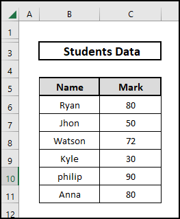
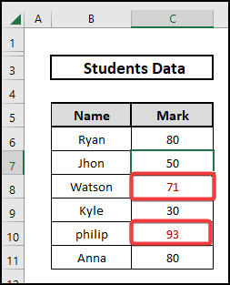
We will explain many approaches to change the text color based on the value in Excel with formulae. For this reason, we have collected a data set of Marksheet of a class containing students’ names and marks.
Unfortunately, there is no built-in Excel function that can alter the text color by itself. Excel’s Conditional Formatting and VBA Macros allow for conditional text coloring. Below, you’ll find three formulas you can use to apply conditional formatting to text in Excel based on a given value.
1. Using ISODD Function with Conditional Formatting
When called, the ISODD function always returns an odd value. With this approach, we’ll utilize an Excel formula based on a function to dynamically alter the text color depending on the value.
⬇️⬇️ STEPS ⬇️⬇️
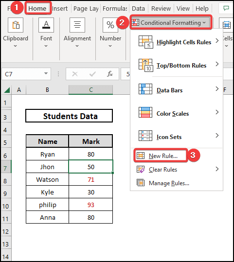
- Select the Home tab option.
- Find the Conditional Formatting option.
- Select the New Rule.
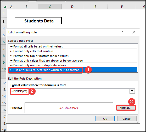
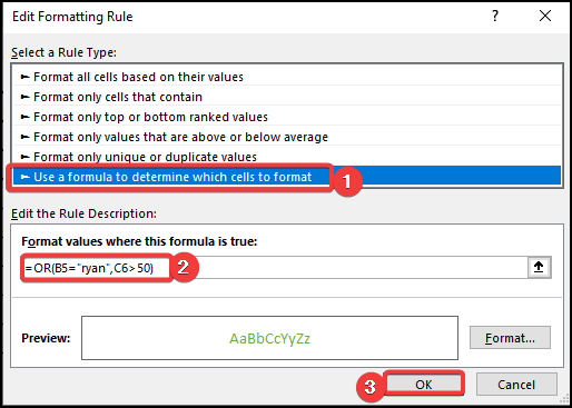
- Select “Use a formula to determine which cells to format”
- Then write down the following formula:
=ISODD(C6)
The function ISODD returns TRUE if the given integer is odd and FALSE otherwise. It will Format the B6 cell if it is odd.
- Then select the Format.
- Preview Color option.
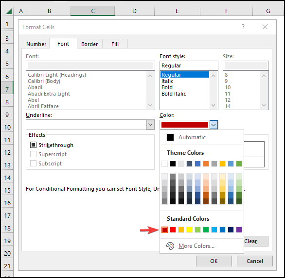
- Finally, select OK.
Then we can see the odd number mark has different formatting.
📕 Read More: 5 Easy Ways to Highlight Highest Value in Excel
2. Apply OR in Conditional Formatting
There will also be an OR operation performed. Here are the measures we need to take.
⬇️⬇️ STEPS ⬇️⬇️
- Repeat the same steps that are followed to set up New Rules.
- Write the following formula:
=OR(B5=”ryan”,C6>50)
🔨 Formula Breakdown
👉 Criteria = OR(B5=”ryan”,C6>50) : The function will separate the value which is more than 50 and if the name is “Ryan“.
- And continue like method 1.
- Later go to the option manage rules and you can see the conditional formatting will be applied in the currently selected range from $C$6 to $C$12.
- And select the OK option to see the output.
As a result, marks greater than 40 are marked as green.
3. Apply COUNTIF Function with Conditional Formatting
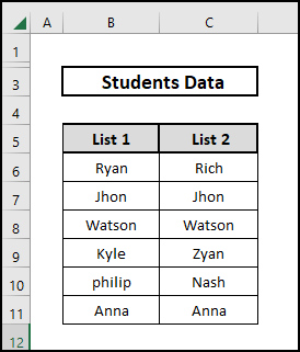
Counting instances that meet specific criteria is the job of the COUNTIF function. We will use this function combined with Conditional Formatting to find common names in two lists that are given below.
⬇️⬇️ STEPS ⬇️⬇️
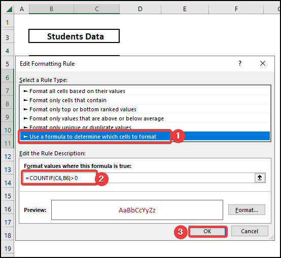
- Apply the New Rule as we did in the previous methods.
- Write down the following formula:
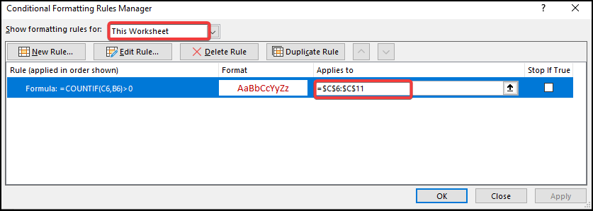
=COUNTIF(C6,B6)>0
🔨 Formula Breakdown
👉 Criteria =COUNTIF(C6,B6)>0 : the function will count entities that exist in both lists.
- And then go to the Option Manage Rules and select the range $C$6:$C$11 and set the formatting drop-in list option for “This Worksheet”.
- Then select OK.
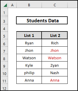
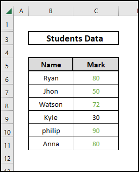
Finally, you will be able to see that the common names in the list are flagged as red.
📕 Read More: Conditional Formatting Dates Older Than Today in Excel
How to Change Color Based on Value of Another Cell in Excel
In the data set, we want to organize it like this, the Name column would be of a different color for the students who scored more than 50.
To accomplish that we followed these steps.
⬇️⬇️ STEPS ⬇️⬇️
- Employ the New Rule as we did in the previous methods.
- Write down the following formula:
=$C6>50
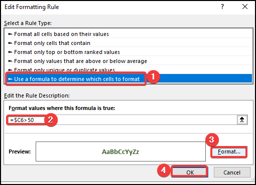
- Then format the cells to Green and Bold.
- See the preview.
- And select the OK option.
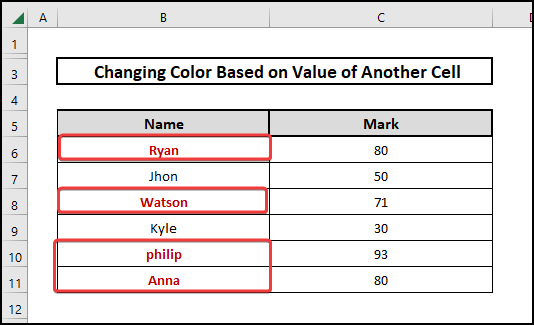
Finally, you can see the students who scored more than 50 are bold with green colors.
📕 Read More: Conditional Formatting Based on Another Cell Date in Excel
Change Font Color Without Conditional Formatting Using VBA in Excel
Now we will change the font color of the cells without conditional formatting by using VBA code. We will Go to the dataset sheet and write the following VBA module:
Sub Colorname()
Dim Roo As Long
Roo = Range("B" & Rows.Count).End(xlUp).Row
For Each cll In Range("B1", "A" & Roo)
    Select Case cll.Value
        Case "Ryan": cll.Offset(0, 1).Font.ColorIndex = 3
        Case "Jhon": cll.Offset(0, 1).Font.ColorIndex = 4
        Case "Anna": cll.Offset(0, 1).Font.ColorIndex = 7
    End Select
Next cll
End Sub
After writing the code output looks like this.
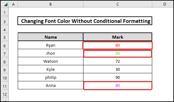
By doing these we can change the font color of the particular text without conditional formatting.
📕 Read More: Excel VBA: If Font Color Is Red Then Return Specific Output
📄 Important Notes
🖊️ Verify that you’ve employed Absolute Reference when it was required. To get an absolute cell reference, press F4.
🖊️ Always look for ways that are easy to use in different situations.
🖊️ Every time you try to use shortcuts on the keyboard.
📝 Takeaways from This Article
📌 You will be able to change color based on odd or even values.
📌 Moreover, you will be able to change color based on certain criteria in the mark sheet, like “pass” or “fail.”
📌 You can verify the common names on two lists.
Conclusion
First and foremost, I hope you were able to apply the principles I taught in this Excel lesson on Excel Formulas to Change Text Color Based on Value. As you can see, there are numerous ways to accomplish this. However, choose the strategy that is best suited to your situation with care. Most essential, if you become confused in any of the processes, I recommend repeating them. After reviewing the Excel file in the practice workbook that I’ve shared above, practice on your own since practice makes perfect. Above all, I sincerely hope you can put it to good use. Please share your thoughts in the comments section about how you felt throughout the article and what we should change or add to make things better for you. However, if you have any Excel-related issues, please leave them in the comments section. The Excelden team is available to answer your inquiries at any time. Finally, keep reading to educate yourself. Please visit our website www.Excelden.com for further Excel-related articles.
Related Articles
- Conditional Formatting to Highlight Dates Within 30 Days in Excel
- 4 Ways to Use Conditional Formatting for Dates Overdue in Excel
- Conditional Formatting to Highlight Row Based on Date in Excel
- 6 Easy Ways to Highlight Lowest Value in Excel
- Conditional Formatting Based on Date Range in Excel


